Time Series Analysis/Forecasting and Univariate ARIMA Models
import os
import sys
import warnings
from datetime import date
import pandas as pd
import pandas_datareader.data as web
import numpy as np
from numpy.linalg import LinAlgError

import statsmodels.tsa.api as tsa
from statsmodels.graphics.tsaplots import plot_acf, acf, plot_pacf, pacf
from statsmodels.tsa.stattools import acf, q_stat, adfuller
import statsmodels.api as sm
from scipy.stats import probplot, moment
from sklearn.metrics import mean_squared_error

import seaborn as sns
import matplotlib.pyplot as plt
import matplotlib as mpl
%matplotlib inline
warnings.filterwarnings('ignore')
sns.set(style="darkgrid", color_codes=True)
def plot_correlogram(x, lags=None, title=None):
    lags = min(10, int(len(x)/5)) if lags is None else lags
    fig, axes = plt.subplots(nrows=2, ncols=2, figsize=(13, 8))
    x.plot(ax=axes[0][0])
    q_p = np.max(q_stat(acf(x, nlags=lags), len(x))[1])
    stats = f'Q-Stat: {np.max(q_p):>8.2f}\nADF: {adfuller(x)[1]:>11.2f}'
    axes[0][0].text(x=.02, y=.85, s=stats, transform=axes[0][0].transAxes)
    probplot(x, plot=axes[0][1])
    mean, var, skew, kurtosis = moment(x, moment=[1, 2, 3, 4])
    s = f'Mean: {mean:>12.2f}\nSD: {np.sqrt(var):>16.2f}\nSkew: {skew:12.2f}\nKurtosis:{kurtosis:9.2f}'
    axes[0][1].text(x=.02, y=.75, s=s, transform=axes[0][1].transAxes)
    plot_acf(x=x, lags=lags, zero=False, ax=axes[1][0])
    plot_pacf(x, lags=lags, zero=False, ax=axes[1][1])
    axes[1][0].set_xlabel('Lag')
    axes[1][1].set_xlabel('Lag')
    fig.suptitle(title, fontsize=20)
    fig.tight_layout()
    fig.subplots_adjust(top=.9)
Download Series
Load monthly Industrial Production and daily NASDAQ stock market index:
industrial_production = web.DataReader('IPGMFN', 'fred', '1988', '2020-02').squeeze().dropna()
nasdaq = web.DataReader('NASDAQCOM', 'fred', '1990', '2020-03-31').squeeze().dropna()
industrial_production
nasdaq
Plot Series
fig, ax = plt.subplots(2,1,figsize=(13, 8))

ax[0].plot(nasdaq, color='b')
ax[1].plot(industrial_production, color='r')

ax[0].set_xlabel('Date')
ax[1].set_xlabel('Date')

ax[0].set_title('NASDAQ', color='b')
ax[1].set_title('Industrial Production', color='r')

ax[0].set_ylabel('NASDAQ Close ($)', color='b')
ax[1].set_ylabel('Production Count', color='r')

ax[0].grid(False)
ax[1].grid(False)

plt.tight_layout()
plt.show()
Additive Decomposition
Time series data typically contains a mix of various patterns that can be decomposed into several components, each representing an underlying pattern category. In particular, time series often consist of the systematic components trend, seasonality and cycles, and unsystematic noise(white noise). These components can be combined in an additive, linear model, in particular when fluctuations do not depend on the level of the series, or in a non-linear, multiplicative model.
These components can be split up automatically. statsmodels includes a simple method to split the time series into a trend, seasonal, and residual component using moving averages. We can apply it to monthly data on industrial manufacturing production with both a strong trend and seasonality component, as follows:
components = tsa.seasonal_decompose(industrial_production, model='additive')
ts = (industrial_production.to_frame('Original')
      .assign(Trend=components.trend)
      .assign(Seasonality=components.seasonal)
      .assign(Residual=components.resid))

ts.plot(subplots=True, figsize=(13, 10))
plt.show()
Time Series Stationarity
The statistical properties, such as the mean, variance, or autocorrelation, of a stationary time series don't change over time. Hence, stationarity implies that a time series does not have any trend or seasonal effects and that descriptive statistics, such as the mean or the standard deviation, when computed for different rolling windows, remain constant or do not change much over time. It reverts to its mean, and the deviations have constant amplitude, while short-term movements always look fairly similar.
Strict stationarity requires the joint distribution of any subset of time series observations to be independent of time with respect to all moments. So, in addition to the mean and variance, higher moments such as skew and kurtosis, also need to be constant, irrespective of the lag between different observations. In most applications, we limit stationarity to first and second moments so that the time series is covariance stationary with constant mean, variance, and autocorrelation.
Note that we specifically allow for dependence between observations at different lags, just like we want the input data for linear regression to be correlated with the outcome. Stationarity implies that these relationships are stable, which facilitates prediction as the model can focus on learning systematic patterns that take place within stable statistical properties.
To satisfy the stationarity assumption of linear time series models, we need to transform the original time series, often in several steps. Common transformations include:
Taking the (natural) logarithm to convert an exponential growth pattern into a linear trend and stabilize the variance.
Deflation implies
dividinga time series by another series that causes trending behavior, for example dividing a nominal series by a price index to convert it into a real measure.Differencing a time-series meaning for each value in the time-series we subtract its previous value.

Other Transformations:
- Take the square root:
np.sqrt(df)
- Take the proportional change:
df.shift(1)/df
Test for stationarity
The augmented Dicky-Fuller test
- Tests for trend non-stationarity
- Null hypothesis is time series is non-stationary
adf = adfuller(industrial_production)

print(f'Test Statistic: {adf[0]}')
print(f'\nP-Value: {adf[1]}')
print(f'\nCritical Values: {adf[4]}')
0thelement is test statistic (-1.59)- More negative means more likely to be stationary
1stelement is p-value: (0.49)- If p-value is small → reject null hypothesis. Reject non-stationary.
4thelement is the critical test statistics
Log Transformation
Check for zero values
(nasdaq == 0).any(), (industrial_production==0).any()
nasdaq_log = np.log(nasdaq)
industrial_production_log = np.log(industrial_production)
Differencing
In many cases, de-trending is not sufficient to make the series stationary. Instead, we need to transform the original data into a series of period-to-period and/or season-to-season differences. Note that when such differencing is applied to a log-transformed series, the results represent instantaneous growth rates or returns in a financial context.
If a univariate series becomes stationary after differencing d times, it is said to be integrated of the order of d, or simply integrated if d=1. This behavior is due to so-called unit roots.
- What is “Unit Root”?
- A unit root (also called a unit root process or a difference stationary process) is a stochastic trend in a time series, sometimes called a “random walk with drift”; If a time series has a unit root, it shows a systematic pattern that is unpredictable.
Differencing of log series produces instantaneous returns.
nasdaq_log_diff = nasdaq_log.diff().dropna()

# seasonal differencing of 12 = yoy instantanteous returns
industrial_production_log_diff = industrial_production_log.diff(12).dropna()
Plot Series
The following chart shows time series for the NASDAQ stock index and industrial production for the 30 years through 2017 in original form, as well as the transformed versions after applying the logarithm and subsequently applying first and seasonal differences (at lag 12), respectively. The charts also display the ADF p-value, which allows us to reject the hypothesis of unit-root non-stationarity after all transformations in both cases:
fig, axes = plt.subplots(nrows=3, ncols=2, figsize=(13,7))

nasdaq.plot(ax=axes[0][0], title='NASDAQ  Composite Index')
axes[0][0].text(x=.03, y=.85, s=f'ADF: {tsa.adfuller(nasdaq.dropna())[1]:.4f}', transform=axes[0][0].transAxes)
axes[0][0].set_ylabel('Index')

nasdaq_log.plot(ax=axes[1][0], sharex=axes[0][0])
axes[1][0].text(x=.03, y=.85, s=f'ADFl: {tsa.adfuller(nasdaq_log.dropna())[1]:.4f}', transform=axes[1][0].transAxes)
axes[1][0].set_ylabel('Log')

nasdaq_log_diff.plot(ax=axes[2][0], sharex=axes[0][0])
axes[2][0].text(x=.03, y=.85, s=f'ADF: {tsa.adfuller(nasdaq_log_diff.dropna())[1]:.4f}', transform=axes[2][0].transAxes)
axes[2][0].set_ylabel('Log, Diff')

industrial_production.plot(ax=axes[0][1], title='Industrial Production: Manufacturing', color='r')
axes[0][1].text(x=.03, y=.85, s=f'ADF: {tsa.adfuller(industrial_production)[1]:.4f}', transform=axes[0][1].transAxes)
axes[0][1].set_ylabel('Index', color='r')

industrial_production_log.plot(ax=axes[1][1], sharex=axes[0][1], color='r')
axes[1][1].text(x=.03, y=.85, s=f'ADF: {tsa.adfuller(industrial_production_log.dropna())[1]:.4f}', transform=axes[1][1].transAxes)
axes[1][1].set_ylabel('Log', color='r')

industrial_production_log_diff.plot(ax=axes[2][1], sharex=axes[0][1], color='r')
axes[2][1].text(x=.83, y=.85, s=f'ADF: {tsa.adfuller(industrial_production_log_diff.dropna())[1]:.4f}', transform=axes[2][1].transAxes)
axes[2][1].set_ylabel('Log, Seasonal Diff', color='r')
fig.tight_layout()
fig.align_ylabels(axes);
Correlogram
Autocorrelation (also called serial correlation) adapts the concept of correlation to the time series context: just as the correlation coefficient measures the strength of a linear relationship between two variables, the autocorrelation coefficient, $\rho_k$, measures the extent of a linear relationship between time series values separated by a given lag, $k$.
Hence, we can calculate one autocorrelation coefficient for each of the T-1 lags in a time series; T is the length of the series. The autocorrelation function (ACF) computes the correlation coefficients as a function of the lags.
The autocorrelation for a lag larger than 1 (that is, between observations more than one time step apart) reflects both the direct correlation between these observations and the indirect influence of the intervening data points.
The partial autocorrelation function (PACF) removes this influence and only measures the linear dependence between data points at the given lag distance. The (PACF) provides all the correlations that result once the effects of correlation at shorter lags have been removed.
A correlogram is simply a plot of the ACF or PACF for sequential lags, k=0,1,...,n. It allows us to inspect the correlation structure across lags at one glance. The main usage of correlograms is to detect any autocorrelation after the removal of the effects of trend or seasonality. Both the ACF and the PACF are key diagnostic tools for the design of linear time series models.

NASDAQ (log, diff)
We can further analyze the relevant time series characteristics for the transformed series using a Q-Q plot that compares the quantiles of the distribution of the time series observation to the quantiles of the normal distribution and the correlograms based on the ACF and PACF.
For the NASDAQ plot, we notice that while there is no trend, the variance is not constant but rather shows clustered spikes around periods of market turmoil in the late 1980s, 2001, and 2008. The Q-Q plot highlights the fat tails of the distribution with extreme values more frequent than the normal distribution would suggest. The ACF and the PACF show similar patterns with autocorrelation at several lags appearing significant:
plot_correlogram(nasdaq_log_diff, lags=100, title='NASDAQ Composite (Log, Diff)')
Industrial Production (log, seasonl diff)
For the monthly time series on industrial manufacturing production, we notice a large negative outlier following the 2008 crisis as well as the corresponding skew in the Q-Q plot. The autocorrelation is much higher than for the NASDAQ returns and declines smoothly. The PACF shows distinct positive autocorrelation patterns at lag 1 and 13, and significant negative coefficients at lags 3 and 4:
plot_correlogram(industrial_production_log_diff, title='Industrial Production (Seasonal Diff)')
Univariate Time Series Models
Autoregressive (AR) Model
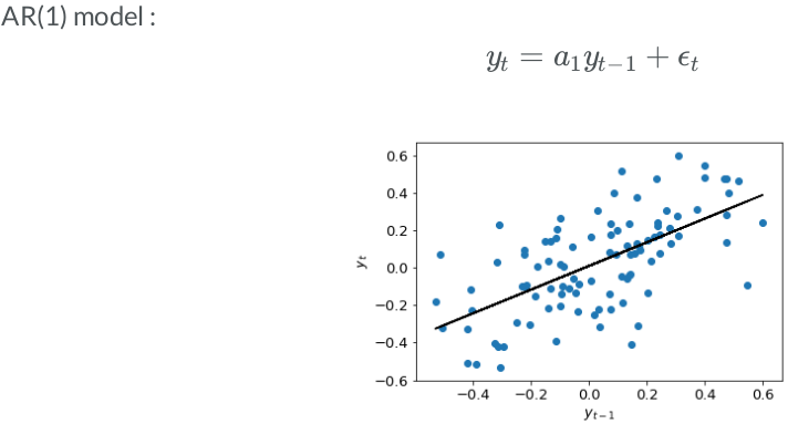
Multiple linear-regression models expressed the variable of interest as a linear combination of predictors or input variables. Univariate time series models relate the value of the time series at the point in time of interest to a linear combination of lagged values of the series and possibly past disturbance terms.
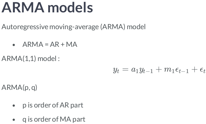
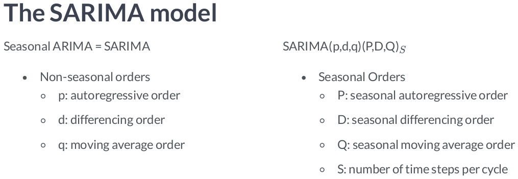
While exponential smoothing models are based on a description of the trend and seasonality in the data, ARIMA models aim to describe the autocorrelations in the data. ARIMA(p, d, q).
- p - number of autoregressive lags
- d - order of differencing
- q - number of moving average lags
Models require stationarity and leverage two building blocks:
- Autoregressive (AR) terms consisting of
p-laggedvalues of the time series

- Moving average (MA) terms that contain
q-laggeddisturbances

ARMA vs ARIMA
The ARMA model of the undifferenced series produces the same result as the ARIMA model of the differenced series.
model1 = tsa.ARMA(endog=nasdaq_log_diff, order=(2,2)).fit()
model2 = tsa.ARIMA(endog=nasdaq_log, order=(2,1,2)).fit()
model1.params.sort_index() == model2.params.sort_index().values
Seasonal differencing vs SARIMAX

Seasonal data
- Has predictable and repeated patterns
- Repeats after any amount of time


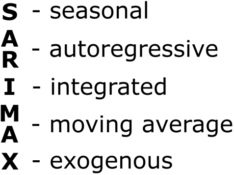
Seasonal differencing has same effect as using SARIMAX with seasonal order (0,1,0,12).
model1 = tsa.statespace.SARIMAX(industrial_production_log, order=(2,0,2), seasonal_order=(0,1,0,12)).fit()
model2 = tsa.statespace.SARIMAX(industrial_production_log_diff, order=(2,0,2), seasonal_order=(0,0,0,12)).fit()
model1.params.to_frame('SARIMAX').join(model2.params.to_frame('diff'))
Finding the optimal ARMA lags
Run candidate models
We iterate over various (p, q) lag combinations and collect diagnostic statistics to compare the result.
train_size = 120 # 10 years of training data
test_results = {}
y_true = industrial_production_log_diff.iloc[train_size:]
for p in range(5):
    for q in range(5):
        aic, bic = [], []
        if p == 0 and q == 0:
            continue
        print(f'p:{p}, q:{q}')
        convergence_error = stationarity_error = 0
        y_pred = []
        for T in range(train_size, len(industrial_production_log_diff)):
            train_set = industrial_production_log_diff.iloc[T-train_size:T]
            try:
                model = tsa.ARMA(endog=train_set, order=(p, q)).fit()
            except LinAlgError:
                convergence_error += 1
            except ValueError:
                stationarity_error += 1

            forecast, _, _ = model.forecast(steps=1)
            y_pred.append(forecast[0])
            aic.append(model.aic)
            bic.append(model.bic)

        result = (pd.DataFrame({'y_true': y_true, 'y_pred': y_pred})
                  .replace(np.inf, np.nan)
                  .dropna())

        rmse = np.sqrt(mean_squared_error(
            y_true=result.y_true, y_pred=result.y_pred))

        test_results[(p, q)] = [rmse,
                                np.mean(aic),
                                np.mean(bic),
                                convergence_error,
                                stationarity_error]
AIC and BIC
AIC = Akaike information criterion
- A Lower AIC indicates a better model
- AIC likes to choose simpler models with a lower order
BIC = Bayesian information criterion
- Very similar to AIC
- A Lower BIC indicates a better model
AIC vs BIC
- BIC favors simpler models than AIC
- AIC is better at choosing predictive models
- BIC is better at choosing good explanatory model
test_results = pd.DataFrame(test_results).T
test_results.columns = ['RMSE', 'AIC', 'BIC', 'convergence', 'stationarity']
test_results.index.names = ['p', 'q']
test_results.info()
# Sort by AIC
test_results.sort_values('AIC').head()
# Sort by BIC
test_results.sort_values('BIC').head()
# Sort by RMSE
test_results.sort_values('RMSE').head()
We aim to minimize RMSE:
sns.heatmap(test_results[['RMSE', 'AIC', 'BIC']].corr('spearman'), fmt='.3', annot=True, cmap='Blues_r')
b, t = plt.ylim()
b += 0.5
t -= 0.5
plt.ylim(b, t)
plt.show()
sns.jointplot(y='RMSE', x='BIC', data=test_results[['RMSE', 'BIC']].rank());
sns.heatmap(test_results.RMSE.unstack().mul(10), fmt='.3', annot=True, cmap='Blues_r')
b, t = plt.ylim()
b += 0.5
t -= 0.5
plt.ylim(b, t)
plt.show()
We also aim to minimize BIC:
sns.heatmap(test_results.BIC.unstack(), fmt='.2f', annot=True, cmap='Blues_r')
b, t = plt.ylim()
b += 0.5
t -= 0.5
plt.ylim(b, t)
plt.show()
Estimating the best ARMA Model
ARMA(0,4) and ARMA(2,2) are close, with a slight edge to ARMA(2,2).
# Just an ARMA(p,q) model
model = tsa.SARIMAX(endog=industrial_production_log_diff, order=(2, 0, 2))

results = model.fit()

print(results.summary())

Plot diagnostics
If the model ts well the residuals will be white Gaussian noise.
# Create the 4 diagostics plots
results.plot_diagnostics(figsize=(13, 8))
plt.show()
Making one-step-ahead predictions
# Make in-sample predictions for last 30 values
forecast = results.get_prediction(start=-30)

# forecast mean
mean_forecast = forecast.predicted_mean

# Get confidence intervals of forecasts
confidence_intervals = forecast.conf_int()

# Select lower and upper confidence limits
lower_limits = confidence_intervals.loc[:,'lower IPGMFN']
upper_limits = confidence_intervals.loc[:,'upper IPGMFN']
Plotting predictions
plt.figure(figsize=(13, 5))

# plot the amazon data
plt.plot(industrial_production_log_diff.dropna().index, industrial_production_log_diff.dropna(), label='observed')

# Plot prediction
plt.plot(mean_forecast.index, mean_forecast.values, color='red', label='forecast')

# Shade uncertainty area
plt.fill_between(confidence_intervals.index, lower_limits, upper_limits, color='pink')

# Calculate MAE
residuals = results.resid
mae = np.mean(np.abs(residuals))

# Calculate RMSE
preds = pd.DataFrame(results.forecasts).T
preds.index = industrial_production_log_diff.dropna().index
preds. columns = ['pred']

rmse = np.sqrt(mean_squared_error(
            y_true=industrial_production_log_diff.dropna(), y_pred=preds.pred))

# set labels, legends and show plot
plt.xlabel('Date')
plt.title(f'Industrial Production MAE = {round(mae,4)}, RMSE = {round(rmse,4)}')
plt.ylabel('Production Count')
plt.margins(0.01)
plt.legend()
plt.show()
Forecasting out of sample
# forecast next 30 days
forecast = results.get_forecast(steps=30)

# forecast mean
mean_forecast = forecast.predicted_mean

# Get confidence intervals of forecasts
confidence_intervals = forecast.conf_int()

# Select lower and upper confidence limits
lower_limits = confidence_intervals.loc[:,'lower IPGMFN']
upper_limits = confidence_intervals.loc[:,'upper IPGMFN']
plt.figure(figsize=(13, 5))

# plot the amazon data
plt.plot(industrial_production_log_diff.dropna().index, industrial_production_log_diff.dropna(), label='observed')

# Plot prediction
plt.plot(mean_forecast.index, mean_forecast.values, color='red', label='forecast')

# Shade uncertainty area
plt.fill_between(confidence_intervals.index, lower_limits, upper_limits, color='pink')

# set labels, legends and show plot
plt.xlabel('Date')
plt.title('Industrial Production')
plt.ylabel('Production Count')
plt.margins(0.01)
plt.legend()
plt.show()
Reconstructing original time series after differencing
diff_forecast = results.get_forecast(steps=30).predicted_mean

from numpy import cumsum

mean_forecast = cumsum(diff_forecast) + pd.DataFrame(industrial_production).iloc[-1,0]
plt.figure(figsize=(13, 5))

# plot the amazon data
plt.plot(industrial_production.index, industrial_production, label='observed')

# Plot prediction
plt.plot(mean_forecast.index, mean_forecast.values, color='red', label='forecast')

# set labels, legends and show plot
plt.xlabel('Date')
plt.title('Industrial Production')
plt.ylabel('Production Count')
plt.margins(x=0.01, y=0.01)
plt.legend()
plt.show()
SARIMAX
model = tsa.SARIMAX(endog=industrial_production_log_diff.dropna(),
                    order=(2, 0, 2),
                    seasonal_order=(1, 0, 1, 12))

results = model.fit(start_params=[0, 0, 0, 0, 0, 0, 1])

print(results.summary())
results.plot_diagnostics(figsize=(13, 8))
plt.show()
# Make in-sample predictions for last 30 values
forecast = results.get_prediction(start=-30)

# forecast mean
mean_forecast = forecast.predicted_mean

# Get confidence intervals of forecasts
confidence_intervals = forecast.conf_int()

# Select lower and upper confidence limits
lower_limits = confidence_intervals.loc[:,'lower IPGMFN']
upper_limits = confidence_intervals.loc[:,'upper IPGMFN']
plt.figure(figsize=(13, 5))

# plot the amazon data
plt.plot(industrial_production_log_diff.dropna().index, industrial_production_log_diff.dropna(), label='observed')

# Plot prediction
plt.plot(mean_forecast.index, mean_forecast.values, color='red', label='forecast')

# Shade uncertainty area
plt.fill_between(confidence_intervals.index, lower_limits, upper_limits, color='pink')

# Calculate MAE
residuals = results.resid
mae = np.mean(np.abs(residuals))

# Calculate RMSE
preds = pd.DataFrame(results.forecasts).T
preds.index = industrial_production_log_diff.dropna().index
preds. columns = ['pred']

rmse = np.sqrt(mean_squared_error(
            y_true=industrial_production_log_diff.dropna(), y_pred=preds.pred))

# set labels, legends and show plot
plt.xlabel('Date')
plt.title(f'Industrial Production MAE = {round(mae,4)}, RMSE = {round(rmse,4)}')
plt.ylabel('Production Count')
plt.margins(0.01)
plt.legend()
plt.show()
We will build a SARIMAX model for monthly data on an industrial production time series for the 1988-2020 period. As illustrated in the first section on analytical tools, the data has been log-transformed, and we are using seasonal (lag-12) differences. We estimate the model for a range of both ordinary and conventional AR and MA parameters and evaluate the RMSE of the 1-step-ahead forecast.
Automation
Searching over model orders to find the optimal number of lags
import pmdarima as pm

results = pm.auto_arima(industrial_production_log_diff.dropna(),

d=0, # non-seasonal difference order
start_p=1, # initial guess for p
start_q=1, # initial guess for q
max_p=3, # max value of p to test
max_q=3, # max value of q to test

seasonal=True, # is the time series seasonal
m=12, # the seasonal period
D=0, # seasonal difference order
start_P=1, # initial guess for P
start_Q=1, # initial guess for Q
max_P=2, # max value of P to test
max_Q=2, # max value of Q to test

information_criterion='bic', # used to select best model
trace=True, # print results whilst training
error_action='ignore', # ignore orders that don't work
stepwise=True, # apply intelligent order search

)
Train best model
results = model.fit()

print(results.summary())
results.plot_diagnostics(figsize=(13, 8))
plt.show()
# Make in-sample predictions for last 30 values
forecast = results.get_prediction(start=-30)

# forecast mean
mean_forecast = forecast.predicted_mean

# Get confidence intervals of forecasts
confidence_intervals = forecast.conf_int()

# Select lower and upper confidence limits
lower_limits = confidence_intervals.loc[:,'lower IPGMFN']
upper_limits = confidence_intervals.loc[:,'upper IPGMFN']
plt.figure(figsize=(13, 5))

# plot the amazon data
plt.plot(industrial_production_log_diff.dropna().index, industrial_production_log_diff.dropna(), label='observed')

# Plot prediction
plt.plot(mean_forecast.index, mean_forecast.values, color='red', label='forecast')

# Shade uncertainty area
plt.fill_between(confidence_intervals.index, lower_limits, upper_limits, color='pink')

# Calculate MAE
residuals = results.resid
mae = np.mean(np.abs(residuals))

# Calculate RMSE
preds = pd.DataFrame(results.forecasts).T
preds.index = industrial_production_log_diff.dropna().index
preds. columns = ['pred']

rmse = np.sqrt(mean_squared_error(
            y_true=industrial_production_log_diff.dropna(), y_pred=preds.pred))

# set labels, legends and show plot
plt.xlabel('Date')
plt.title(f'Industrial Production MAE = {round(mae,4)}, RMSE = {round(rmse,4)}')
plt.ylabel('Production Count')
plt.margins(0.01)
plt.legend()
plt.show()