Non-negative matrix factorization
NMF= "non-negative matrix factorization"- Dimension reduction technique
- NMF models are interpretable (unlike PCA)
- Easy to interpret and easy to explain!
- However, all sample features must be non-negative
(>= 0)
Using scikit-learn NMF
- Follows fit() / transform() pa!ern
- Must specify number of components e.g. NMF(n_components=2)
- Works with NumPy arrays and with csr_matrix
NMF components
- NMF has components
- ... just like PCA has principal components
- Dimension of components = dimension of samples
- Entries are non-negative
from sklearn.decomposition import NMF
from sklearn.feature_extraction.text import TfidfVectorizer
from sklearn import datasets

iris = datasets.load_iris()
samples = iris.data

model = NMF(n_components=2)

model.fit(samples)

nmf_features = model.transform(samples)

print(model.components_)
NMF features
- NMF feature values are non-negative
- Can be used to reconstruct the samples
- ... combine feature values with components
print(nmf_features[:5])
Sample reconstruction
- Multiply components by feature values, and add up
- Can also be expressed as a product of matrices
- This is the "Matrix Factorization" in "NMF"
NMF fits to non-negative data, only
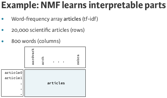
- Word frequencies in each document
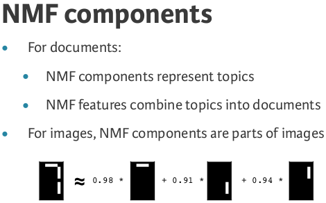
- Images encoded as arrays
- Audio spectrograms
- Purchase histories on e-commerce sites
- ... and many more!
print(samples[0, :])

#multiplying components by feature values and add up (dot product)
print(nmf_features[0, :].dot(model.components_))
import pandas as pd

df = pd.read_csv("data/wikipedia_articles_to_cluster.csv",  encoding = "ISO-8859-1")
titles = df.title

df.head()
from sklearn.feature_extraction.text import TfidfVectorizer

# Create a TfidfVectorizer: tfidf
tfidf = TfidfVectorizer()

# Apply fit_transform to document: csr_mat
articles = tfidf.fit_transform(df.article_text.values)
# Create an NMF instance: model
model = NMF(n_components=6)

# Fit the model to articles
model.fit(articles)

# Transform the articles: nmf_features
nmf_features = model.transform(articles)

# Print the NMF features
print(nmf_features[:5])
NMF features of the Wikipedia articles
# Create a pandas DataFrame: df
df = pd.DataFrame(nmf_features, index=titles)

# Print the row for 'Anne Hathaway'
print(df.loc['Anne Hathaway'])

# Print the row for 'Denzel Washington'
print(df.loc['Denzel Washington'])
When investigating the features, notice that for both actors, the NMF feature 1 has by far the highest value. This means that both articles are reconstructed using mainly the 1st NMF component.
# Create a DataFrame: components_df
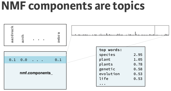
components_df = pd.DataFrame(model.components_)

# Print the shape of the DataFrame
print(components_df.shape)

# Select row 3: component
component = components_df.iloc[3]

# Print result of nlargest
print(component.nlargest())
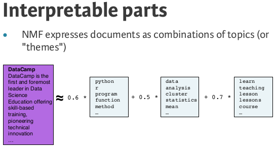
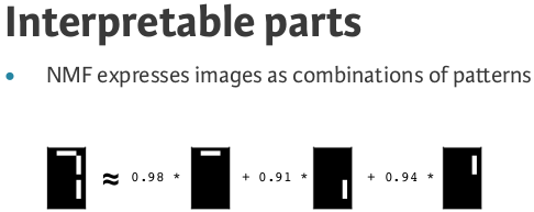
NMF learns interpretable parts / Topic-modeling
Working with a grayscale images = no colors ony shades of gray measuring pixel brightness beteen 0 and 1
def show_as_image(vector):
    """
    Given a 1d vector representing an image, display that image in
    black and white.  If there are negative values, then use red for
    that pixel.
    """
    bitmap = vector.reshape((13, 8))  # make a square array
    bitmap /= np.abs(vector).max()  # normalise
    bitmap = bitmap[:,:,np.newaxis]
    rgb_layers = [np.abs(bitmap)] + [bitmap.clip(0)] * 2
    rgb_bitmap = np.concatenate(rgb_layers, axis=-1)
    plt.imshow(rgb_bitmap, cmap='gray', interpolation='nearest')
    plt.xticks([])
    plt.yticks([])
    plt.colorbar()
    plt.show()
digit_7 = np.array([0.,  0.,  0.,  0.,  0.,  0.,  0.,  0.,
                    0.,  0.,  1.,  1.,  1.,  1.,  0.,  0.,
                    0.,  0.,  0.,  0.,  0.,  0.,  1.,  0.,
                    0.,  0.,  0.,  0.,  0.,  0.,  1.,  0.,
                    0.,  0.,  0.,  0.,  0.,  0.,  1.,  0.,
                    0.,  0.,  0.,  0.,  0.,  0.,  1.,  0.,
                    0.,  0.,  0.,  0.,  0.,  0.,  0.,  0.,
                    0.,  0.,  0.,  0.,  0.,  0.,  1.,  0.,
                    0.,  0.,  0.,  0.,  0.,  0.,  1.,  0.,
                    0.,  0.,  0.,  0.,  0.,  0.,  1.,  0.,
                    0.,  0.,  0.,  0.,  0.,  0.,  1.,  0.,
                    0.,  0.,  0.,  0.,  0.,  0.,  0.,  0.,
                    0.,  0.,  0.,  0.,  0.,  0.,  0.,  0.])

show_as_image(digit_7)
NMF learns the parts of images
Now we will use NMF to decompose the digits dataset.
samples = np.loadtxt('data/lcd-digits.csv', delimiter=',')

# Create an NMF model: model
model = NMF(n_components=7)

# Apply fit_transform to samples: features
features = model.fit_transform(samples)

# Call show_as_image on each component
for component in model.components_:
    show_as_image(component)

# Assign the 0th row of features: digit_features
digit_features = features[0,:]
# Print digit_features
print(digit_features)
PCA doesn't learn parts
Unlike NMF, PCA doesn't learn the parts of things. Its components do not correspond to topics (in the case of documents) or to parts of images, when trained on images. We verify this for by inspecting the components of a PCA model fit to the dataset.
# Import PCA
from sklearn.decomposition import PCA

# Create a PCA instance: model
model = PCA(n_components=7)

# Apply fit_transform to samples: features
features = model.fit_transform(samples)

# Call show_as_image on each component
for component in model.components_:
    show_as_image(component)
Finding similar articles
- Engineer at a large online newspaper
- Task: recommend articles similar to article being read by customers
- Similar articles should have similar topics
Strategy
- Apply NMF to the word-frequency array
- NMF feature values describe the topics
- ... so similar documents have similar NMF feature values
- Compare NMF feature values?
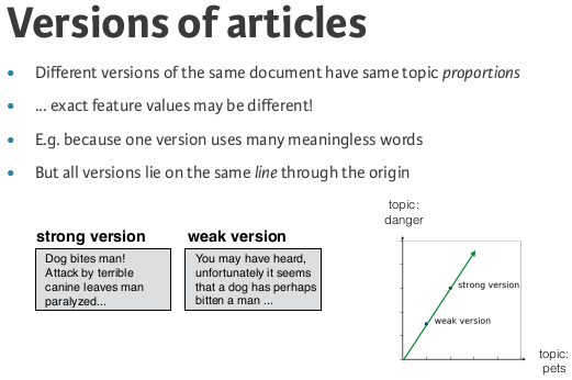
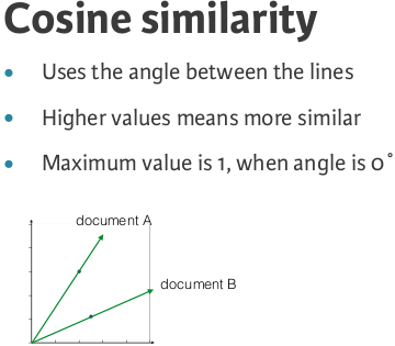
Cosine similarityis a metric used to measure how similar the documents are irrespective of their size. Mathematically, it measures the cosine of the angle between two vectors projected in a multi-dimensional space. The cosine similarity is advantageous because even if the two similar documents are far apart by the Euclidean distance (due to the size of the document), chances are they may still be oriented closer together. The smaller the angle, higher the cosine similarity.
Which articles are similar to 'Cristiano Ronaldo'?
We will be finding the articles most similar to the article about the footballer Cristiano Ronaldo using NMF features and the cosine similarity to find similar articles.
Building recommender systems using NMF
- Finding similar artciles
- Recommend articles similar to one being read
- Strategy : apply NMF to word-frequencey array
- NMF features values describe the topics (similar artcile have similar NMF features values)
nmf = NMF(n_components=6)

#apply NMF to word frequence array
nmf_features = nmf.fit_transform(articles)

# Normalize the NMF features: norm_features
norm_features = normalize(nmf_features)

# Create a DataFrame: df
df = pd.DataFrame(norm_features, index=titles)

# Select the row corresponding to 'Cristiano Ronaldo': article
article = df.loc['Cristiano Ronaldo']

# Compute the dot products: similarities
similarities = df.dot(article)

# Display those with the largest cosine similarity
print(similarities.nlargest())
