Market Basket Analysis in Python
Amazon, Netflix and many other popular companies rely on Market Basket Analysis to produce meaningful product recommendations. Market Basket Analysis is a powerful tool for translating vast amounts of customer transaction and viewing data into simple rules for product promotion and recommendation. In this notebook, we’ll learn how to perform Market Basket Analysis using the Apriori algorithm, standard and custom metrics, association rules, aggregation and pruning, and visualization.
What is market basket analysis?
- Identify products frequently purchased together.
- Bookstore Ex:
- Biography and history
- Fiction and poetry
- Construct recommendations based on these
- Bookstore Ex:
- Place biography and history sections together.
- Keep fiction and history apart
The use cases of market basket analysis
- Build Netflix-style recommendations engine.
- Improve product recommendations on an e-commerce store.
- Cross-sell products in a retail setting.
- Improve inventory management.
- Upsell products.
- Market basket analysis
- Construct association rules
- Identify items frequently purchased together
- Association rules
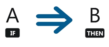
- {antecedent}→{consequent}
- {fiction}→{biography}
- {antecedent}→{consequent}
Imports
import numpy as np
import pandas as pd
import matplotlib.pyplot as plt
import seaborn as sns
from mlxtend.frequent_patterns import apriori
from mlxtend.frequent_patterns import association_rules
sns.set(style="darkgrid", color_codes=True)
pd.set_option('display.max_columns', 75)
Dataset
The contains information about customers buying different grocery items.
data = pd.read_csv('Market_Basket.csv', header = None)
data.info()
data.head()
data.describe()
EDA
color = plt.cm.rainbow(np.linspace(0, 1, 40))
data[0].value_counts().head(40).plot.bar(color = color, figsize=(13,5))
plt.title('frequency of most popular items', fontsize = 20)
plt.xticks(rotation = 90 )
plt.grid()
plt.show()
import networkx as nx
data['food'] = 'Food'
food = data.truncate(before = -1, after = 15)
food = nx.from_pandas_edgelist(food, source = 'food', target = 0, edge_attr = True)
import warnings
warnings.filterwarnings('ignore')

plt.rcParams['figure.figsize'] = (13, 13)
pos = nx.spring_layout(food)
color = plt.cm.Set1(np.linspace(0, 15, 1))
nx.draw_networkx_nodes(food, pos, node_size = 15000, node_color = color)
nx.draw_networkx_edges(food, pos, width = 3, alpha = 0.6, edge_color = 'black')
nx.draw_networkx_labels(food, pos, font_size = 20, font_family = 'sans-serif')
plt.axis('off')
plt.grid()
plt.title('Top 15 First Choices', fontsize = 20)
plt.show()
Getting the list of transactions
Once we have read the dataset, we need to get the list of items in each transaction. SO we will run two loops here. One for the total number of transactions, and other for the total number of columns in each transaction. This list will work as a training set from where we can generate the list of association rules.
# Getting the list of transactions from the dataset
transactions = []
for i in range(0, len(data)):
    transactions.append([str(data.values[i,j]) for j in range(0, len(data.columns))])
transactions[:1]
Association rules
- Association rule
- Contains antecedent and consequent
- {health} → {cooking}
- Contains antecedent and consequent
- Multi-antecedent rule
- {humor, travel} → {language}
- Multi-consequent rule
- {biography} → {history, language}
- Multi-antecedent and consequent rule
- {biography, non-fiction} → {history, language}
Difficulty of selecting rules
- Finding useful rules is difficult.
- Set of all possible rules is large.
- Most rules are not useful.
- Must discard most rules.
- What if we restrict ourselves to simple rules?
- One antecedent and one consequent.
- Still challenging, even for small dataset.
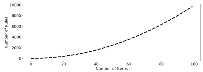
As the number of items increase the number of rules increases exponentially.
from itertools import permutations

# Extract unique items.
flattened = [item for transaction in transactions for item in transaction]
items = list(set(flattened))
print('# of items:',len(items))
print(list(items))
if 'nan' in items: items.remove('nan')
print(list(items))
# Compute and print rules.
rules = list(permutations(items, 2))
print('# of rules:',len(rules))
print(rules[:5])
One-hot encoding transaction data
Throughout we will use a common pipeline for preprocessing data for use in market basket analysis. The first step is to import a pandas DataFrame and select the column that contains transactions. Each transaction in the column will be a string that consists of a number of items, each separated by a comma. The next step is to use a lambda function to split each transaction string into a list, thereby transforming the column into a list of lists. Then we will transform the transactions into a one-hot encoded DataFrame, where each column consists of TRUE and FALSE values that indicate whether an item was included in a transaction.
# Import the transaction encoder function from mlxtend
from mlxtend.preprocessing import TransactionEncoder

# Instantiate transaction encoder and identify unique items
encoder = TransactionEncoder().fit(transactions)

# One-hot encode transactions
onehot = encoder.transform(transactions)

# Convert one-hot encoded data to DataFrame
onehot = pd.DataFrame(onehot, columns = encoder.columns_).drop('nan', axis=1)

# Print the one-hot encoded transaction dataset
onehot.head()
Metrics and pruning
- A metric is a measure of performance for rules.
- {humor} → {poetry}
- 0.81
- {fiction} → {travel}
- 0.23
- {humor} → {poetry}
- Pruning is the use of metrics to discard rules.
- Retain: {humor} → {poetry}
- Discard: { ction} → {travel}
The simplest metric
- The support metric measures the share of transactions that contain an itemset.
# Compute the support
support = onehot.mean()
support = pd.DataFrame(support, columns=['support']).sort_values('support',ascending=False)

# Print the support
support.head()
support.describe()
Confidence and lift
When support is misleading
- Milk and bread frequently purchased together.
- Support: {Milk} → {Bread}
- Rule is not informative for marketing.
- Milk and bread are both independently popular items.
The confidence metric
- Can improve over support with additional metrics.
- Adding confidence provides a more complete picture.
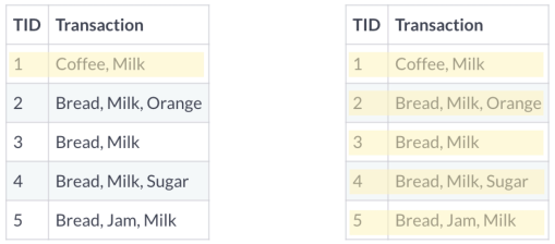
- Confidence gives us the probability we will purchase $Y$ given we have purchased $X$.
Interpreting the confidence metric
 $$\text{Support(Milk&Coffee)} = 0.20$$
- The probability of purchasing both milk and coffee does not change if we condition on purchasing milk. Purchasing milk tells us nothing about purchasing coffee.
The lift metric
- Lift provides another metric for evaluating the relationship between items.
- Numerator: Proportion of transactions that contain $X$ and $Y$.
- Denominator: Proportion if $X$ and $Y$ are assigned randomly and independently to transactions.
- Lift $> 1$ tells us $2$ items occur in transactions together more often than we would expect based on their individual support values. This means the relationship is unlikely to be explained by random chance. This natural threshold is convenient for filtering purposes.
- Lift $< 1$ tells us $2$ items are paired together less frequently in transactions than we would expect if the pairings occurred by random chance.
Recommending food with support
A grocery-store wants to get members to eat more and has decided to use market basket analysis to figure out how. They approach you to do the analysis and ask that you use the five most highly-rated food items.
# Compute support for burgers and french fries
supportBF = np.logical_and(onehot['burgers'], onehot['french fries']).mean()

# Compute support for burgers and mineral water
supportBM = np.logical_and(onehot['burgers'], onehot['mineral water']).mean()

# Compute support for french fries and mineral water
supportFM = np.logical_and(onehot['french fries'], onehot['mineral water']).mean()

# Print support values
print("burgers and french fries: %.2f" % supportBF)
print("burgers and mineral water: %.2f" % supportBM)
print("french fries and mineral water: %.2f" % supportFM)
Computing the support metric
Previously we one-hot encoded a small grocery store's transactions as the DataFrame onehot. In this exercise, we'll make use of that DataFrame and the support metric to help the store's owner. First, she has asked us to identify frequently purchased items, which we'll do by computing support at the item-level. And second, she asked us to check whether the rule {mineral water} → {french fries} has a support of over $0.05$.
# Add a mineral water+french fries column to the DataFrame onehot
onehot['mineral water+french fries'] = np.logical_and(onehot['mineral water'], onehot['french fries'])

# Compute the support
support = onehot.mean()
val = support.loc['mineral water+french fries']

# Print the support values
print(f'mineral water+french fries support = {val}')
Refining support with confidence
After reporting your findings from the previous exercise, the store's owner asks us about the direction of the relationship. Should they use mineral water to promote french fries or french fries to promote mineral water?
We decide to compute the confidence metric, which has a direction, unlike support. We'll compute it for both {mineral water} → {french fries} and {french fries} → {mineral water}.
# Compute support for mineral water and french fries
supportMF = np.logical_and(onehot['mineral water'], onehot['french fries']).mean()

# Compute support for mineral water
supportM = onehot['mineral water'].mean()

# Compute support for french fries
supportF = onehot['french fries'].mean()

# Compute confidence for both rules
confidenceMM = supportMF / supportM
confidenceMF = supportMF / supportF

# Print results
print('mineral water = {0:.2f}, french fries = {1:.2f}'.format(confidenceMM, confidenceMF))
Even though the support is identical for the two association rules, the confidence is much higher for french fries -> mineral water, since french fries has a higher support than mineral water.
Further refinement with lift
Once again, we report our results to the store's owner: Use french fries to promote mineral water, since the rule has a higher confidence metric. The store's owner thanks us for the suggestion, but asks us to confirm that this is a meaningful relationship using another metric.
You recall that lift may be useful here. If lift is less than $1$, this means that mineral water and french fries are paired together less frequently than we would expect if the pairings occurred by random chance.
# Compute lift
lift = supportMF / (supportM * supportF)

# Print lift
print("Lift: %.2f" % lift)
As it turns out, lift is less than $1.0$. This does not give us good confidence that the association rule we recommended did not arise by random chance.
Leverage and Conviction
The leverage metric
Leverage also builds on support. $$ \text{Leverage}(X \rightarrow Y ) = $$
$$ \text{Support}(X\&Y) − \text{Support}(X)\text{Support}(Y) $$- Leverage is similar to lift, but easier to interpret.
- Leverage lies in $-1$ and $+1$ range.
- Lift ranges from $0$ to infinity.
The conviction metric
- Conviction is also built using support.
- More complicated and less intuitive than leverage. $$ \text{Conviction}(X \rightarrow Y) = $$
Computing conviction
The store's owner asks us if we are able to compute conviction for the rule {burgers} → {french fries}, so she can decide whether to place the items next to each other on the company's website.
# Compute support for burgers AND french fries
supportBF = np.logical_and(onehot['burgers'], onehot['french fries']).mean()

# Compute support for burgers
supportB = onehot['burgers'].mean()

# Compute support for NOT french fries
supportnF = 1.0 - onehot['french fries'].mean()

# Compute support for burgers and NOT french fries
supportBnF = supportB - supportBF

# Compute and print conviction for burgers -> french fries
conviction = supportB * supportnF / supportBnF
print("Conviction: %.2f" % conviction)
Notice that the value of conviction was greater than $1$, suggesting that the rule if burgers then french fries is supported.
Computing conviction with a function
The store's owner asks us if we are able to compute conviction for every pair of food items in the grocery-store dataset, so she can use that information to decide which food items to locate closer together on the website.
We agree to take the job, but realize that we a need more efficient way to compute conviction, since we will need to compute it many times. We decide to write a function that computes it. It will take two columns of a pandas DataFrame as an input, one antecedent and one consequent, and output the conviction metric.
def conviction(antecedent, consequent):
    # Compute support for antecedent AND consequent
    supportAC = np.logical_and(antecedent, consequent).mean()

    # Compute support for antecedent
    supportA = antecedent.mean()

    # Compute support for NOT consequent
    supportnC = 1.0 - consequent.mean()

    # Compute support for antecedent and NOT consequent
    supportAnC = supportA - supportAC

    # Return conviction
    return supportA * supportnC / supportAnC
Computing leverage with a function
def leverage(antecedent, consequent):
    # Compute support for antecedent AND consequent
    supportAB = np.logical_and(antecedent, consequent).mean()

    # Compute support for antecedent
    supportA = antecedent.mean()

    # Compute support for consequent
    supportB = consequent.mean()

    # Return leverage
    return supportAB - supportB * supportA
Promoting food with conviction
Previously we defined a function to compute conviction. We were asked to apply that function to all two-food items permutations of the grocery-store dataset. We'll test the function by applying it to the three most popular food items, which we used in earlier exercises: burgers, french fries, and mineral water.
# Compute conviction for burgers -> french fries and french fries -> burgers
convictionBF = conviction(onehot['burgers'], onehot['french fries'])
convictionFB = conviction(onehot['french fries'], onehot['burgers'])

# Compute conviction for burgers -> mineral water and mineral water -> burgers
convictionBM = conviction(onehot['burgers'], onehot['mineral water'])
convictionMB = conviction(onehot['mineral water'], onehot['burgers'])

# Compute conviction for french fries -> mineral water and mineral water -> french fries
convictionFM = conviction(onehot['french fries'], onehot['mineral water'])
convictionMF = conviction(onehot['mineral water'], onehot['french fries'])

# Print results
print('french fries -> burgers: ', convictionFB)
print('burgers -> french fries: ', convictionBF)
Association and Dissociation
Zhang's metric
- Introduced by Zhang(2000)
- Takes values between $-1$ and $+1$
- Value of $+1$ indicates perfect association
- Value of $-1$ indicates perfect dissociation
- Comprehensive and interpretable
- Constructed using support
Defining Zhang's metric
$$ \text{Zhang}(A \rightarrow B) = $$$$ \frac{\text{Confidence}(A \rightarrow B) − \text{Confidence}( \bar{A} \rightarrow B)}{\max(\text{Confidence}(A \rightarrow B), \text{Confidence}( \bar{A} \rightarrow B))} $$$$ \text{Confidence} = \frac{\text{Support}(A\&B)}{\text{Support}(A)}$$- Using only support
Computing association and dissociation
The store's owner has returned to you once again about your recommendation to promote french fries using burgers. They're worried that the two might be dissociated, which could have a negative impact on their promotional effort. They ask you to verify that this is not the case.
You immediately think of Zhang's metric, which measures association and dissociation continuously. Association is positive and dissociation is negative.
# Compute the support of burgers and french fries
supportT = onehot['burgers'].mean()
supportP = onehot['french fries'].mean()

# Compute the support of both food items
supportTP = np.logical_and(onehot['burgers'], onehot['french fries']).mean()

# Complete the expressions for the numerator and denominator
numerator = supportTP - supportT*supportP
denominator = max(supportTP*(1-supportT), supportT*(supportP-supportTP))

# Compute and print Zhang's metric
zhang = numerator / denominator
print(zhang)
Once again, the association rule if burgers then french fries proved robust. It had a positive value for Zhang's metric, indicating that the two food items are not dissociated.
Defining Zhang's metric
In general, when we want to perform a task many times, we'll write a function, rather than coding up each individual instance. In this exercise, we'll define a function for Zhang's metric that takes an antecedent and consequent and outputs the metric itself.
# Define a function to compute Zhang's metric
def zhang(antecedent, consequent):
    # Compute the support of each book
    supportA = antecedent.mean()
    supportC = consequent.mean()

    # Compute the support of both books
    supportAC = np.logical_and(antecedent, consequent).mean()

    # Complete the expressions for the numerator and denominator
    numerator = supportAC - supportA*supportC
    denominator = max(supportAC*(1-supportA), supportA*(supportC-supportAC))

    # Return Zhang's metric
    return numerator / denominator
Applying Zhang's metric
The store's owner has sent you a list of itemsets she's investigating and has asked us to determine whether any of them contain items that are dissociated. When we're finished, she has asked that us to add the metric we use to a column in the rules DataFrame.
# Create rules DataFrame
rules_ = pd.DataFrame(rules, columns=['antecedents','consequents'])

# Define an empty list for metrics
zhangs, conv, lev, antec_supp, cons_supp, suppt, conf, lft = [], [], [], [], [], [], [], []

# Loop over lists in itemsets
for itemset in rules:
    # Extract the antecedent and consequent columns
    antecedent = onehot[itemset[0]]
    consequent = onehot[itemset[1]]

    antecedent_support = onehot[itemset[0]].mean()
    consequent_support = onehot[itemset[1]].mean()
    support = np.logical_and(onehot[itemset[0]], onehot[itemset[1]]).mean()
    confidence = support / antecedent_support
    lift = support / (antecedent_support * consequent_support)

    # Complete metrics and append it to the list
    antec_supp.append(antecedent_support)
    cons_supp.append(consequent_support)
    suppt.append(support)
    conf.append(confidence)
    lft.append(lift)
    lev.append(leverage(antecedent, consequent))
    conv.append(conviction(antecedent, consequent))
    zhangs.append(zhang(antecedent, consequent))

# Store results
rules_['antecedent support'] = antec_supp
rules_['consequent support'] = cons_supp
rules_['support'] = suppt
rules_['confidence'] = conf
rules_['lift'] = lft
rules_['leverage'] = lev
rules_['conviction'] = conv
rules_['zhang'] = zhangs

# Print results
rules_.sort_values('zhang',ascending=False).head()
rules_.describe()
rules_.info()
Notice that most of the items were dissociated, which suggests that they would have been a poor choice to pair together for promotional purposes.
Overview of market basket analysis
Standard procedure for market basket analysis.
- Generate large set of rules.
- Filter rules using metrics.
- Apply intuition and common sense.
Filtering with support and conviction
The store's owner has approached you with the DataFrame rules, which contains the work of a data scientist who was previously on staff. It includes columns for antecedents and consequents, along with the performance for each of those rules with respect to a number of metrics.
Our objective will be to perform multi-metric filtering on the dataset to identify potentially useful rules.
# Select the subset of rules with antecedent support greater than 0.05
rules_filtered = rules_[rules_['antecedent support'] > 0.05]

# Select the subset of rules with a consequent support greater than 0.01
rules_filtered = rules_[rules_['consequent support'] > 0.01]

# Select the subset of rules with a conviction greater than 1.01
rules_filtered = rules_[rules_['conviction'] > 1.01]

# Select the subset of rules with a lift greater than 1.0
rules_filtered = rules_[rules_['lift'] > 1.0]

# Print remaining rules
print(f'# of rules = {len(rules_)}')
print(f'# of rules after filtering = {len(rules_filtered)}')
print(rules_filtered.head())
Using multi-metric filtering to cross-promote food items
As a final request, the store's owner asks us to perform additional filtering. Our previous attempt returned $8598$ rules, but she wanted much less.
# Set the threshold for Zhang's rule to 0.65
rules_filtered = rules_filtered[rules_filtered['zhang'] > 0.65]

# Print rule
print(f'# of rules after filtering = {8598 - len(rules_filtered)}')
print(rules_filtered.head())
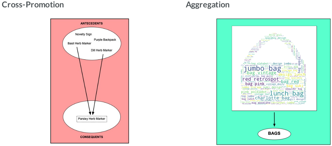
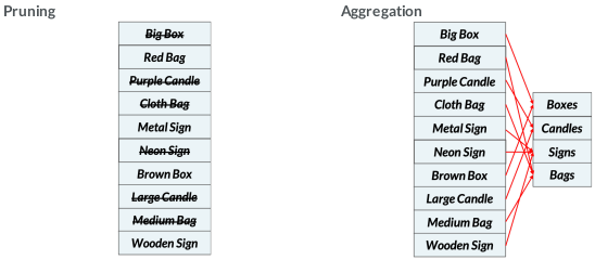
Aggregation
Novelty gift data
url = 'https://assets.datacamp.com/production/repositories/5654/datasets/5a3bc2ebccb77684a6d8a9f3fbec23fe04d4e3aa/online_retail.csv'
gifts = pd.read_csv(url)
gifts.info()
gifts.head()
# Stripping extra spaces in the description
gifts['Description'] = gifts['Description'].str.strip()
# Dropping the rows without any invoice number
gifts.dropna(subset =['InvoiceNo'], inplace = True)
gifts['InvoiceNo'] = gifts['InvoiceNo'].astype('str')
# Dropping all transactions which were done on credit
gifts = gifts[~gifts['InvoiceNo'].str.contains('C')]
EDA
# Print number of transactions.
print(len(gifts['InvoiceNo'].unique()))
# Print number of items.
print(len(gifts['Description'].unique()))
# Recover unique InvoiceNo's.
InvoiceNo = gifts['InvoiceNo'].unique()

# Create basket of items for each transaction.
Transactions = [list(gifts[gifts['InvoiceNo'] == u].Description.astype(str)) for u in InvoiceNo]
# Print example transaction.
Transactions[0]
# Instantiate transaction encoder.
encoder = TransactionEncoder()

# One-hot encode transactions.
onehot = encoder.fit(Transactions).transform(Transactions)

# Use unique items as column headers.
onehot = pd.DataFrame(onehot, columns = encoder.columns_).drop('nan', axis=1)

# Print onehot header.
onehot.head()
Performing aggregation
After completing minor consulting jobs we've finally received our first big market basket analysis project: advising an online novelty gifts retailer on cross-promotions. Since the retailer has never previously hired a data scientist, they would like you to start the project by exploring its transaction data. They have asked us to perform aggregation for all signs in the dataset and also compute the support for this category.
# Convert words to a list of words
def convert_str(string):
    lst = list(string.split(' '))
    return lst
# Select the column headers for sign items
sign_headers = []
for i in onehot.columns:
    wrd_lst = convert_str(str(i).lower())
    if 'sign' in wrd_lst:
        sign_headers.append(i)
# Select columns of sign items
sign_columns = onehot[sign_headers]

# Perform aggregation of sign items into sign category
signs = sign_columns.sum(axis = 1) >= 1.0

# Print support for signs
print('Share of Signs: %.2f' % signs.mean())
Defining an aggregation function
Surprised by the high share of sign items in its inventory, the retailer decides that it makes sense to do further aggregation for different categories to explore the data better. This seems trivial to us, but the retailer has not previously been able to perform even a basic descriptive analysis of its transaction and items.
The retailer asks us to perform aggregation for the candles, bags, and boxes categories. To simplify the task, we decide to write a function. It will take a string that contains an item's category. It will then output a DataFrame that indicates whether each transaction includes items from that category.
def aggregate(item):
    # Select the column headers for sign items
    item_headers = []
    for i in onehot.columns:
        wrd_lst = convert_str(str(i).lower())
        if item in wrd_lst:
            item_headers.append(i)

    # Select columns of sign items
    item_columns = onehot[item_headers]

    # Return category of aggregated items
    return item_columns.sum(axis = 1) >= 1.0
# Aggregate items for the bags, boxes, and candles categories
bags = aggregate('bag')
boxes = aggregate('box')
candles = aggregate('candle')

print('Share of Bags: %.2f' % bags.mean())
print('Share of Boxes: %.2f' % boxes.mean())
print('Share of Candles: %.2f' % candles.mean())
The Apriori algorithm
Counting itemsets
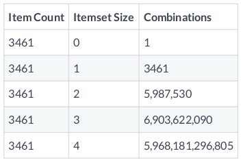
$$ \begin{pmatrix} n \\ k \end{pmatrix} = \frac{n!}{(n - k)!k!} $$$$ \sum_{k=1}^n \begin{pmatrix} n \\ k \end{pmatrix} = 2^n $$- $n = 3461 \rightarrow 2^{3461}$
- $2^{3461} >> 10^{82}$
- Number of atoms in universe: $10^{82}$.
Reducing the number of itemsets
- Not possible to consider all itemsets.
- Not even possible to enumerate them.
- How do we remove an itemset without even evaluating it?
- Could set maximum $k$ value.
- Apriori algorithm offers alternative.
- Doesn't require enumeration of all itemsets.
- Sensible rule for pruning.
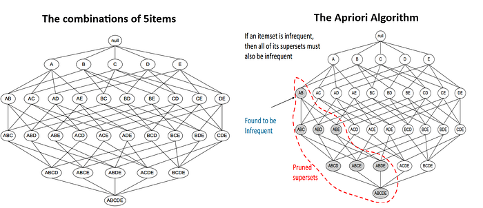
The Apriori principle
- Apriori principle.
- Subsets of frequent sets are frequent.
- Retain sets known to be frequent.
- Prune sets not known to be frequent.
Ex:
- Candles = Infrequent
- -> {Candles, Signs} = Infrequent
- {Candles, Signs} = Infrequent
- -> {Candles, Signs Boxes} = Infrequent
- {Candles, Signs, Boxes} = Infrequent
- -> {Candles, Signs, Boxes, Bags} = Infrequent
Identifying frequent itemsets with Apriori
The aggregation exercise we performed for the online retailer proved helpful. It offered a starting point for understanding which categories of items appear frequently in transactions. The retailer now wants to explore the individual items themselves to find out which are frequent.
Here we'll apply the Apriori algorithm to the online retail dataset without aggregating first. Our objective will be to prune the itemsets using a minimum value of support and a maximum item number threshold.
# Import apriori from mlxtend
from mlxtend.frequent_patterns import apriori

# Compute frequent itemsets using the Apriori algorithm
frequent_itemsets = apriori(onehot,
                            min_support = 0.05,
                            max_len = 3,
                            use_colnames = True)

# Print a preview of the frequent itemsets
frequent_itemsets.head()
Selecting a support threshold
The manager of the online gift store looks at the results we provided from the previous exercise and commends us for the good work. She does, however, raise an issue: all of the itemsets we identified contain only one item. She asks whether it would be possible to use a less restrictive rule and to generate more itemsets, possibly including those with multiple items.
After agreeing to do this, we think about what might explain the lack of itemsets with more than $1$ item. It can't be the max_len parameter, since that was set to $3$. We decide it must be support and decide to test two different values, each time checking how many additional itemsets are generated.
# Import apriori from mlxtend
from mlxtend.frequent_patterns import apriori

# Compute frequent itemsets using a support of 0.04 and length of 3
frequent_itemsets_1 = apriori(onehot, min_support = 0.04,
                            max_len = 3, use_colnames = True)

# Compute frequent itemsets using a support of 0.05 and length of 3
frequent_itemsets_2 = apriori(onehot, min_support = 0.05,
                            max_len = 3, use_colnames = True)

# Print the number of freqeuent itemsets
print(len(frequent_itemsets_1), len(frequent_itemsets_2))
Basic Apriori results pruning
- Apriori prunes itemsets.
- Applies minimum support threshold.
- Modi ed version can prune by number of items.
- Doesn't tell us about association rules.
- Association rules.
- Many more association rules than itemsets.
- {Bags, Boxes}: Bags -> Boxes OR Boxes -> Bags.
How to compute association rules
- Computing rules from Apriori results.
- Difficult to enumerate for high $n$ and $k$.
- Could undo itemset pruning by Apriori.
- Reducing number of association rules.
mlxtendmodule offers means of pruning association rules.association_rules()takes frequent items, metric, and threshold.
Generating association rules
Previously we computed itemsets for the novelty gift store owner using the Apriori algorithm. You told the store owner that relaxing support from 0.05 to 0.04 increased the number of itemsets from $50$ to $87$. Satisfied with the descriptive work we've done, the store manager asks us to identify some association rules from those two sets of frequent itemsets we computed.
Our objective is to determine what association rules can be mined from these itemsets.
# Import the association rule function from mlxtend
from mlxtend.frequent_patterns import association_rules

# Compute all association rules for frequent_itemsets_1
rules_1 = association_rules(frequent_itemsets_1,
                            metric = "support",
                            min_threshold = 0.001)

# Compute all association rules for frequent_itemsets_2
rules_2 = association_rules(frequent_itemsets_2,
                            metric = "support",
                            min_threshold = 0.002)

# Print the number of association rules generated
print(len(rules_1), len(rules_2))
Pruning with lift
Once again, we report back to the novelty gift store manager. This time, we tell her that we identified $2$ rules when you used a higher support threshold for the Apriori algorithm and only $6$ rules when you used a lower threshold. She commends us for the good work, but asks you to consider using another metric to refine the two rules.
You remember that lift had a simple interpretation: values greater than $1$ indicate that items co-occur more than we would expect if they were independently distributed across transactions. We decide to use lift, since that message will be simple to convey.
# Import the association rules function
from mlxtend.frequent_patterns import association_rules

# Compute frequent itemsets using the Apriori algorithm
frequent_itemsets = apriori(onehot, min_support = 0.03,
                            max_len = 2, use_colnames = True)

# Compute all association rules for frequent_itemsets
rules = association_rules(frequent_itemsets,
                            metric = "lift",
                            min_threshold = 1.0)

# Print association rules
rules.info()
rules.head()
Pruning with confidence
We decide to see whether pruning by another metric might allow us to narrow things down even further.
What would be the right metric? Both lift and support are identical for all rules that can be generated from an itemset, so we decide to use confidence instead, which differs for rules produced from the same itemset.
# Import the association rules function
from mlxtend.frequent_patterns import apriori, association_rules

# Compute frequent itemsets using the Apriori algorithm
frequent_itemsets = apriori(onehot, min_support = 0.03,
                            max_len = 2, use_colnames = True)

# Compute all association rules using confidence
rules = association_rules(frequent_itemsets,
                            metric = "confidence",
                            min_threshold = 0.4)

# Print association rules
rules.info()
rules.head()
Aggregation and filtering
The store manager is now asking us to generate a floorplan proposal, where each pair of sections should contain one high support product and one low support product.
# Aggregate items
signs = aggregate('sign')

# Concatenate aggregated items into 1 DataFrame
aggregated = pd.concat([bags, boxes, candles, signs],axis=1)
aggregated.columns = ['bag','box','candle','sign']

# Apply the apriori algorithm with a minimum support of 0.04
frequent_itemsets = apriori(aggregated, min_support = 0.04, use_colnames = True)

# Generate the initial set of rules using a minimum support of 0.01
rules = association_rules(frequent_itemsets,
                          metric = "support", min_threshold = 0.01)

# Set minimum antecedent support to 0.35
rules = rules[rules['antecedent support'] > 0.35]

# Set maximum consequent support to 0.35
rules = rules[rules['consequent support'] < 0.35]

# Print the remaining rules
rules.info()
rules.head()
Applying Zhang's rule
We learned that Zhang's rule is a continuous measure of association between two items that takes values in the $-1,+1$ interval. A $-1$ value indicates a perfectly negative association and a $+1$ value indicates a perfectly positive association. In this exercise, we'll determine whether Zhang's rule can be used to refine a set of rules a gift store is currently using to promote products.
We will start by re-computing the original set of rules. After that, we will apply Zhang's metric to select only those rules with a high and positive association.
# Funtion to compute Zhang's rule from mlxtend association_rules output
def zhangs_rule(rules):
    PAB = rules['support'].copy()
    PA = rules['antecedent support'].copy()
    PB = rules['consequent support'].copy()
    NUMERATOR = PAB - PA*PB
    DENOMINATOR = np.max((PAB*(1-PA).values,PA*(PB-PAB).values), axis = 0)
    return NUMERATOR / DENOMINATOR
# Generate the initial set of rules using a minimum lift of 1.00
rules = association_rules(frequent_itemsets, metric = "lift", min_threshold = 1.00)

# Set antecedent support to 0.04
rules = rules[rules['antecedent support'] > 0.04]

# Set consequent support to 0.04
rules = rules[rules['consequent support'] > 0.04]

# Compute Zhang's rule
rules['zhang'] = zhangs_rule(rules)

# Set the lower bound for Zhang's rule to 0.5
rules = rules[rules['zhang'] > 0.5]
rules[['antecedents', 'consequents']].info()
rules.tail()
Advanced filtering with multiple metrics
Earlier, we used data from an online novelty gift store to find antecedents that could be used to promote a targeted consequent. Since the set of potential rules was large, we had to rely on the Apriori algorithm and multi-metric filtering to narrow it down. In this exercise, we'll examine the full set of rules and find a useful one, rather than targeting a particular antecedent.
In this exercise, we'll apply the Apriori algorithm to identify frequent itemsets. We'll then recover the set of association rules from the itemsets and apply multi-metric filtering.
# Apply the Apriori algorithm with a minimum support threshold of 0.04
frequent_itemsets = apriori(onehot, min_support = 0.04, use_colnames = True)

# Recover association rules using a minium support threshold of 0.01
rules = association_rules(frequent_itemsets, metric = 'support', min_threshold = 0.01)

# Apply a 0.002 antecedent support threshold, 0.01 confidence threshold, and 2.50 lift threshold
filtered_rules = rules[(rules['antecedent support'] > 0.002) &
                       (rules['consequent support'] > 0.01) &
                       (rules['confidence'] > 0.60) &
                       (rules['lift'] > 2.50)]

# Print remaining rule
filtered_rules[['antecedents','consequents']]
Movielens dataset
The data consists of $105339$ ratings applied over $10329$ movies. There are $668$ users who has given their ratings for $149532$ movies.
movie_raitings = pd.read_csv('movie_raitings.csv', index_col = 'Unnamed: 0')
movie_raitings = movie_raitings[movie_raitings['rating'] >= 4.0]
movie_raitings.info()
movie_raitings.head()
# Recover unique user IDs.
user_id = movie_raitings['userId'].unique()

# Create library of  movies for each user.
libraries = [list(movie_raitings[movie_raitings['userId'] == u].title) for u in user_id]

# Print example library.
print(libraries[0])
# Instantiate transaction encoder.
encoder = TransactionEncoder()

# One-hot encode libraries.
onehot = encoder.fit(libraries).transform(libraries)

# Use movie titles as column headers.
onehot = pd.DataFrame(onehot, columns = encoder.columns_)

# Print onehot header.
onehot.head()
Visualizing itemset support
A content-streaming start-up has approached us for consulting services. To keep licensing fees low, they want to assemble a narrow library of movies that all appeal to the same audience. While they'll provide a smaller selection of content than the big players in the industry, they'll also be able to offer a low subscription fee.
We decide to use the MovieLens data and a heatmap for this project. Using a simple support-based heatmap will allow us to identify individual titles that have high support with other titles.
# Apply the apriori algorithm
frequent_itemsets = apriori(onehot, min_support=0.15, use_colnames=True, max_len=2)

# Recover the association rules
rules = association_rules(frequent_itemsets)

rules.info()
rules.head()
Heatmaps
- Heatmaps help us understand a large number of rules between a small number of antecedents and consequents
# Convert antecedents and consequents into strings
rules['antecedents'] = rules['antecedents'].apply(lambda a: ','.join(list(a)))
rules['consequents'] = rules['consequents'].apply(lambda a: ','.join(list(a)))

# Transform antecedent, consequent, and support columns into matrix
support_table = rules.pivot(index='consequents', columns='antecedents', values='support')

plt.figure(figsize=(10,6))
sns.heatmap(support_table, annot=True, cbar=False)
b, t = plt.ylim()
b += 0.5
t -= 0.5
plt.ylim(b, t)
plt.yticks(rotation=0)
plt.show()
Heatmaps with lift
The founder likes the heatmap we've produced for her streaming service. After discussing the project further, however, we decide that that it is important to examine other metrics before making a final decision on which movies to license. In particular, the founder suggests that we select a metric that tells us whether the support values are higher than we would expect given the films' individual support values.
We recall that lift does this well and decide to use it as a metric. We also remember that lift has an important threshold at $1.0$ and decide that it is important to replace the colorbar with annotations, so you can determine whether a value is greater than $1.0$.
# Import seaborn under its standard alias
import seaborn as sns

# Transform the DataFrame of rules into a matrix using the lift metric
pivot = rules.pivot(index = 'consequents',
                    columns = 'antecedents', values= 'lift')

# Generate a heatmap with annotations on and the colorbar off
plt.figure(figsize=(10,6))
sns.heatmap(pivot, annot = True, cbar = False)
b, t = plt.ylim()
b += 0.5
t -= 0.5
plt.ylim(b, t)
plt.yticks(rotation=0)
plt.xticks(rotation=90)
plt.show()
Scatterplots
- Scatter plots will help us to evaluate general tendencies and behaviors of rules between many antecedents and consequents but, without isolating any rule in particular.
- A scatterplot displays pairs of values.
- Antecedent and consequent support.
- Confidence and lift.
- No model is assumed.
- No trend line or curve needed.
- Can provide starting point for pruning.
- Identify patterns in data and rules.
What can we learn from scatterplots?
- Identify natural thresholds in data.
- Not possible with heatmaps or other visualizations.
- Visualize entire dataset.
- Not limited to small number of rules.
- Use findings to prune.
- Use natural thresholds and patterns to prune.
Pruning with scatterplots
After viewing your streaming service proposal from the previous exercise, the founder realizes that her initial plan may have been too narrow. Rather than focusing on initial titles, she asks you to focus on general patterns in the association rules and then perform pruning accordingly. Our goal should be to identify a large set of strong associations.
Fortunately, we've just learned how to generate scatterplots. We decide to start by plotting support and confidence, since all optimal rules according to many common metrics are located on the confidence-supply border.
## Apply the Apriori algorithm with a support value of 0.0095
frequent_itemsets = apriori(onehot, min_support = 0.0095,
                            use_colnames = True, max_len = 2)

# Generate association rules without performing additional pruning
rules = association_rules(frequent_itemsets, metric='support',
                          min_threshold = 0.0)

# Generate scatterplot using support and confidence
plt.figure(figsize=(10,6))
sns.scatterplot(x = "support", y = "confidence", data = rules)
plt.margins(0.01,0.01)
plt.show()
Notice that the confidence-support border roughly forms a triangle. This suggests that throwing out some low support rules would also mean that we would discard rules that are strong according to many common metrics.
Optimality of the support-confidence border
We return to the founder with the scatterplot produced in the previous exercise and ask whether she would like us to use pruning to recover the support-confidence border. We tell her about the Bayardo-Agrawal result, but she seems skeptical and asks whether we can demonstrate this in an example.
Recalling that scatterplots can scale the size of dots according to a third metric, we decide to use that to demonstrate optimality of the support-confidence border. We will show this by scaling the dot size using the lift metric, which was one of the metrics to which Bayardo-Agrawal applies.
# Generate scatterplot using support and confidence
plt.figure(figsize=(10,6))
sns.scatterplot(x = "support", y = "confidence",
                size = "lift", data = rules)
plt.margins(0.01,0.01)
plt.show()
If you look at the plot carefully, you'll notice that the highest values of lift are always at the support-confidence border for any given value of confidence.
Parallel coordinates plot
- The parallel coordinates plot will allow us to visualize whether a relationship exist between an antecedent and consequent. We can think of it as a directed network diagram. The plot shows connections between $2$ objects that are related and indicates the direction of the relationship.
When to use parallel coordinate plots
- Parallel coordinates vs. heatmap.
- Don't need intensity information.
- Only want to know whether rule exists.
- Want to reduce visual clutter.
- Parallel coordinates vs. scatterplot.
- Want individual rule information.
- Not interested in multiple metrics.
- Only want to examine final rules.
Using parallel coordinates to visualize rules
Our visual demonstration in the previous exercise convinced the founder that the supply-confidence border is worthy of further exploration. She now suggests that we extract part of the border and visualize it. Since the rules that fall on the border are strong with respect to most common metrics, she argues that we should simply visualize whether a rule exists, rather than the intensity of the rule according to some metric. We realize that a parallel coordinates plot is ideal for such cases.
# Function to convert rules to coordinates.
def rules_to_coordinates(rules):
    rules['antecedent'] = rules['antecedents'].apply(lambda antecedent: list(antecedent)[0])
    rules['consequent'] = rules['consequents'].apply(lambda consequent: list(consequent)[0])
    rules['rule'] = rules.index
    return rules[['antecedent','consequent','rule']]
from pandas.plotting import parallel_coordinates

# Compute the frequent itemsets
frequent_itemsets = apriori(onehot, min_support = 0.15,
                            use_colnames = True, max_len = 2)

# Compute rules from the frequent itemsets
rules = association_rules(frequent_itemsets, metric = 'confidence',
                          min_threshold = 0.55)

# Convert rules into coordinates suitable for use in a parallel coordinates plot
coords = rules_to_coordinates(rules)

# Generate parallel coordinates plot
plt.figure(figsize=(4,8))
parallel_coordinates(coords, 'rule')
plt.legend([])
plt.grid(True)
plt.show()
