Introduction to A/B testing

What is A/B testing?
- A/B Testing: Test different ideas against each other in the real world
- Choose the one that statistically performs better
Why is A/B testing important?
- No guessing
- Provides accurate answers - quickly
- Allows to rapidly iterate on ideas and establish causal relationships
A/B test process
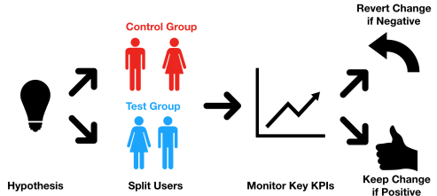
- Develop a hypothesis about your product or business
- Randomly assign users to two different groups
- Expose:
- Group 1 to the the current product rules
- Group 2 to a product that tests the hypothesis
Where can A/B testing be used?
- impact of drugs
- incentivizing spending
- driving user growth
- ...and many more!
- Pick whichever performs better according to a set of KPIs Key Performance Indicators
Key performance indicators (KPIs)
A/B Tests: Measure impact of changes on KPIs
- KPIs — metrics are important to an organization:
- likelihood of a side-effect
- revenue
- conversion rate
How to identify KPIs
Experience + Domain knowledge + Exploratory data analysis
Experience & Knowledge - What is important to a business
Exploratory Analysis - What metrics and relationships impact these KPIs
Imports
import warnings
warnings.filterwarnings('ignore')
import pandas as pd
import numpy as np
import matplotlib.pyplot as plt
import seaborn as sns
from functools import reduce
from sklearn import preprocessing
from scipy import stats
Control and treatment (test) groups
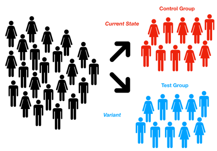
Testing two or more ideas against each other:
- Control: The current state of your product
- Treatment(s): The variant(s) that you want to test
Our problem
A/B Test - improving our app paywall
Question: Which paywall has a higher conversion rate?
- Current Paywall: ”I hope you enjoyed your free-trial, please consider subscribing” (control)
- Proposed Paywall: “Your free-trial has ended, don’t miss out, subscribe today!” (treatment)
A/B testing process
- Randomly subset the users and show one set the control and one the treatment
- Monitor the conversion rates of each group to see which is better
The importance of randomness
- Random assignment helps to...
- isolate the impact of the change made
- reduce the potential impact of confounding variables
- Using an assignment criteria may introduce confounders
Good problems for A/B testing
- Users are impacted individually
- Testing changes that can directly impact their behavior
Bad problems for A/B testing
- Cases with network effects among users
- Challenging to segment the users into groups
- Difficult to untangle the impact of the test
Our data set
We are looking at data from an app. The app is very simple and has just $4$ pages:
The first page is the home page. When you come to the site for the first time, you can only land on the home page as a first page.
From the home page, the user can perform a search and land on the search page.
From the search page, if the user clicks on a product, she will get to the payment page (paywall), where she is asked to provide payment information in order to subscribe.
If she does decide to buy, she ends up on the confirmation page
Data set overview
We have $5$ files, $4$ of them contains page_visit information and $1$ of them contains user information.
- page_visit_information
- home_page_table.csv
- search_page_table.csv
- payment_page_table.csv
- payment_confirmation_table.csv
- user_information page
- user_table.csv
Create test and control groups
user_table = pd.read_csv('user_table.csv')
length = len(user_table['user_id'])
k = np.random.binomial(1, 0.495, length)
user_table['group'] = k
user_table['group'] = user_table['group'].replace(False, 'Control', regex=True)
user_table['group'] = user_table['group'].replace(True, 'Test', regex=True)
user_table.head()
Merging
Merge all csv files together by user_id.
# Read in all csv files
home_page_table = pd.read_csv('home_page_table.csv')
search_page_table = pd.read_csv('search_page_table.csv')
payment_page_table = pd.read_csv('payment_page_table.csv')
payment_confirmation_table = pd.read_csv('payment_confirmation_table.csv')

# Compile the list of dataframes you want to merge
data_frames = [user_table, home_page_table, search_page_table, payment_page_table, payment_confirmation_table]

# Merge all dataframes in the list together on user_id
df_merged = reduce(lambda  left,right: pd.merge(left,right,on=['user_id'], how='outer'), data_frames)
df_merged.columns = ['user_id', 'date', 'device', 'sex', 'group', 'home_page', 'search_page',
                     'payment_page', 'payment_confirm']
df_merged.info()
Data Preprocessing
We create $4$ new columns indicating whether a user is in home_page, search_page, payment_page, confirmation_page, $1$ indicating that one person is in this page and $0$ other wise.
df_merged['date'] = pd.to_datetime(df_merged['date'])

trans_features = df_merged[['home_page', 'search_page', 'payment_page', 'payment_confirm']]
trans_features = trans_features.replace(np.nan, 'none', regex=True)
other_features = df_merged[['user_id', 'date', 'device', 'sex', 'group']]

le = preprocessing.LabelEncoder()
trans_features = trans_features.apply(lambda x: le.fit_transform(x))

df_merged = pd.concat([other_features, trans_features], axis=1)
df_merged['home_page'] = df_merged['home_page'].replace(0, 1)
Poisson distribution
The Poisson distribution is a discrete probability distribution that expresses the probability of a given number of events occurring in a fixed interval of time or space if these events occur with a known constant rate and independently of the time since the last event. The Poisson distribution can also be used for the number of events in other specified intervals such as distance, area or volume.
- For instance the number of phone calls received by a call center per hour may obeys a Poisson distribution.
- The Poisson distribution is a limit of the Binomial distribution for rare events.
Ideally, payment_confirm (binary outcome of a customer subscribing) should be a Poisson distribution. There will be customers with no subscription and we will have less customers that subscribe. Let’s use numpy.random.poisson() for assigning different distributions to the test and control group
test_n = len(df_merged.loc[df_merged.group == 'Test'])
cont_n = len(df_merged.loc[df_merged.group == 'Control'])
df_merged.loc[df_merged.group == 'Test', 'payment_confirm'] = np.random.poisson(0.089, test_n)
df_merged.loc[df_merged.group == 'Control', 'payment_confirm'] = np.random.poisson(0.079, cont_n)
df_merged.info()
df_merged.head()
Grouping and aggregating our combined dataset
daily_purchase_data = df_merged.groupby(by=['date'], as_index=False)
daily_purchase_data = daily_purchase_data.agg({'payment_confirm': ['sum', 'count']})
daily_purchase_data.columns = daily_purchase_data.columns.droplevel(level=0)
daily_purchase_data.columns = ['date', 'sum', 'count']

Male = df_merged[df_merged.sex == 'Male']
Female = df_merged[df_merged.sex == 'Female']

Desktop = df_merged[df_merged.device == 'Desktop']
Mobile = df_merged[df_merged.device == 'Mobile']

Male_Desktop = Male[Male.device == 'Desktop']
Male_Mobile = Male[Male.device == 'Mobile']

Female_Desktop = Female[Female.device == 'Desktop']
Female_Mobile = Female[Female.device == 'Mobile']

Male_daily_purchase_data = Male.groupby(by=['date'], as_index=False)
Male_daily_purchase_data = Male_daily_purchase_data.agg({'payment_confirm': ['sum', 'count']})
Male_daily_purchase_data.columns = Male_daily_purchase_data.columns.droplevel(level=0)
Male_daily_purchase_data.columns = ['date', 'sum', 'count']

Female_daily_purchase_data = Female.groupby(by=['date'], as_index=False)
Female_daily_purchase_data = Female_daily_purchase_data.agg({'payment_confirm': ['sum', 'count']})
Female_daily_purchase_data.columns = Female_daily_purchase_data.columns.droplevel(level=0)
Female_daily_purchase_data.columns = ['date', 'sum', 'count']

Desktop_daily_purchase_data = Desktop.groupby(by=['date'], as_index=False)
Desktop_daily_purchase_data = Desktop_daily_purchase_data.agg({'payment_confirm': ['sum', 'count']})
Desktop_daily_purchase_data.columns = Desktop_daily_purchase_data.columns.droplevel(level=0)
Desktop_daily_purchase_data.columns = ['date', 'sum', 'count']

Mobile_daily_purchase_data = Mobile.groupby(by=['date'], as_index=False)
Mobile_daily_purchase_data = Mobile_daily_purchase_data.agg({'payment_confirm': ['sum', 'count']})
Mobile_daily_purchase_data.columns = Mobile_daily_purchase_data.columns.droplevel(level=0)
Mobile_daily_purchase_data.columns = ['date', 'sum', 'count']

daily_visitor_data = df_merged.groupby(by=['date'], as_index=False)
daily_visitor_data = daily_visitor_data.agg({'home_page': ['sum', 'count']})
daily_visitor_data.columns = daily_visitor_data.columns.droplevel(level=0)
daily_visitor_data.columns = ['date', 'sum', 'count']

daily_visitor_Male = Male.groupby(by=['date'], as_index=False)
daily_visitor_Male = daily_visitor_Male.agg({'home_page': ['sum', 'count']})
daily_visitor_Male.columns = daily_visitor_Male.columns.droplevel(level=0)
daily_visitor_Male.columns = ['date', 'sum', 'count']

daily_visitor_Female = Female.groupby(by=['date'], as_index=False)
daily_visitor_Female = daily_visitor_Female.agg({'home_page': ['sum', 'count']})
daily_visitor_Female.columns = daily_visitor_Female.columns.droplevel(level=0)
daily_visitor_Female.columns = ['date', 'sum', 'count']

daily_visitor_Desktop = Desktop.groupby(by=['date'], as_index=False)
daily_visitor_Desktop = daily_visitor_Desktop.agg({'home_page': ['sum', 'count']})
daily_visitor_Desktop.columns = daily_visitor_Desktop.columns.droplevel(level=0)
daily_visitor_Desktop.columns = ['date', 'sum', 'count']

daily_visitor_Mobile = Mobile.groupby(by=['date'], as_index=False)
daily_visitor_Mobile = daily_visitor_Mobile.agg({'home_page': ['sum', 'count']})
daily_visitor_Mobile.columns = daily_visitor_Mobile.columns.droplevel(level=0)
daily_visitor_Mobile.columns = ['date', 'sum', 'count']

daily_visitor_Mobile_Female = Female_Mobile.groupby(by=['date'], as_index=False)
daily_visitor_Mobile_Female = daily_visitor_Mobile_Female.agg({'home_page': ['sum', 'count']})
daily_visitor_Mobile_Female.columns = daily_visitor_Mobile_Female.columns.droplevel(level=0)
daily_visitor_Mobile_Female.columns = ['date', 'sum', 'count']

daily_visitor_Desktop_Female = Female_Desktop.groupby(by=['date'], as_index=False)
daily_visitor_Desktop_Female = daily_visitor_Desktop_Female.agg({'home_page': ['sum', 'count']})
daily_visitor_Desktop_Female.columns = daily_visitor_Desktop_Female.columns.droplevel(level=0)
daily_visitor_Desktop_Female.columns = ['date', 'sum', 'count']

daily_visitor_Mobile_Male = Male_Mobile.groupby(by=['date'], as_index=False)
daily_visitor_Mobile_Male = daily_visitor_Mobile_Male.agg({'home_page': ['sum', 'count']})
daily_visitor_Mobile_Male.columns = daily_visitor_Mobile_Male.columns.droplevel(level=0)
daily_visitor_Mobile_Male.columns = ['date', 'sum', 'count']

daily_visitor_Desktop_Male = Male_Desktop.groupby(by=['date'], as_index=False)
daily_visitor_Desktop_Male = daily_visitor_Desktop_Male.agg({'home_page': ['sum', 'count']})
daily_visitor_Desktop_Male.columns = daily_visitor_Desktop_Male.columns.droplevel(level=0)
daily_visitor_Desktop_Male.columns = ['date', 'sum', 'count']
EDA
fig, ax = plt.subplots(nrows=2, ncols=2, figsize=(13,8))

ax[0,0].plot(daily_visitor_data['date'], daily_visitor_data['count'], color='b', linestyle='-', marker='o')
ax[0,1].plot(daily_visitor_data['date'], daily_visitor_data['count'].rolling(3).std(), color='r',
           linestyle='-', marker='o')

ax[1,0].plot(daily_visitor_Female['date'], daily_visitor_Female['count'], color='r', linestyle='-', marker='o',
             label='Female')
ax[1,0].plot(daily_visitor_Male['date'], daily_visitor_Male['count'], color='b', linestyle='-', marker='o',
             label='Male')

ax[1,1].plot(daily_visitor_Desktop['date'], daily_visitor_Desktop['count'], color='b', linestyle='-', marker='o',
           label='Desktop')
ax[1,1].plot(daily_visitor_Mobile['date'], daily_visitor_Mobile['count'], color='r', linestyle='-', marker='o',
           label='Mobile')

ax[1,0].set_xlabel('Date', fontsize=14)
ax[1,1].set_xlabel('Date', fontsize=14)
ax[0,1].set_ylabel('Count Std', fontsize=14)
ax[0,0].set_ylabel('Count', fontsize=14)
ax[1,1].set_ylabel('Count', fontsize=14)
ax[1,0].set_ylabel('Count', fontsize=14)
ax[1,0].legend()
ax[1,1].legend()
fig.autofmt_xdate()
plt.tight_layout()
fig.suptitle(f'Daily Visitors', fontsize=24)
plt.subplots_adjust(top=.9)
plt.show()
fig, ax = plt.subplots(nrows=1, ncols=2, figsize=(13,5))
ax[0].plot(daily_purchase_data['date'], daily_purchase_data['sum'], color='b', linestyle='-', marker='o')
ax[1].plot(daily_purchase_data['date'], daily_purchase_data['count'], color='r', linestyle='-', marker='o')
ax[0].set_xlabel('Date', fontsize=14)
ax[1].set_xlabel('Date', fontsize=14)
ax[0].set_ylabel('Sum', fontsize=14)
ax[1].set_ylabel('Count', fontsize=14)
fig.autofmt_xdate()
plt.tight_layout()
fig.suptitle(f'Daily Payment Confirmations', fontsize=24)
plt.subplots_adjust(top=.9)
plt.show()
fig, ax = plt.subplots(nrows=1, ncols=2, figsize=(13,5))
ax[0].plot(Male_daily_purchase_data['date'], Male_daily_purchase_data['count'], color='b', label='Male',
           linestyle='-', marker='o')
ax[0].plot(Female_daily_purchase_data['date'], Female_daily_purchase_data['count'], color='r', label='Female',
           linestyle='-', marker='o')
ax[1].plot(Desktop_daily_purchase_data['date'], Desktop_daily_purchase_data['count'], color='g',
           label='Desktop', linestyle='-', marker='o')
ax[1].plot(Mobile_daily_purchase_data['date'], Mobile_daily_purchase_data['count'], color='y', label='Mobile',
           linestyle='-', marker='o')
ax[0].set_xlabel('Date', fontsize=14)
ax[1].set_xlabel('Date', fontsize=14)
ax[0].set_ylabel('Sex Count', fontsize=14)
ax[1].set_ylabel('Device Count', fontsize=14)
ax[0].legend(bbox_to_anchor=(1.22, 1.02))
ax[1].legend(bbox_to_anchor=(1.24, 1.02))
plt.tight_layout()
fig.suptitle(f'Daily Payment Confirmations', fontsize=24)
plt.subplots_adjust(top=.9)
fig.autofmt_xdate()
plt.show()
# Group and aggregate our combined dataset
grouped_purchase_data = df_merged.groupby(by = ['device', 'sex'])
purchase_summary = grouped_purchase_data.agg({'payment_confirm': ['sum', 'count']})
purchase_summary.head()
Initial A/B test design
Response variable
- The quantity used to measure the impact of your change
- Should either be a KPI or directly related to a KPI
- The easier to measure the better
Factors & variants
- Factors: The type of variable you are changing
- The paywall customer greeting
- Variants: Particular changes you are testing
- Current Paywall: “I hope you enjoyed your free-trial, please consider subscribing” (control)
- Proposed Paywall: “Your free-trial has ended, don’t miss out, subscribe today!” (treatment)
KPI: Conversion Rate
Conversion Rate: Percentage of users who subscribe after the free trial
Across all users or just a subset?
Of users who convert within one week? One month?
Why is conversion rate important?
- Strong measure of growth
- Potential early warning sign of problems
- Sensitive to changes in the overall ecosystem
- Choosing a KPI
- Stability over time
- Importance across different user groups
- Correlation with other business factors
Conversion rate sensitivities
Here were working with the conversion rate metric. Specifically we will work to examine what that value becomes under different percentage lifts and look at how many more conversions per day this change would result in. First we will find the average number of paywall views and purchases that were made per day in our observed sample.
# Find the mean of each field and then multiply by 1000 to scale the result
daily_purchases = daily_purchase_data['sum'].mean()
daily_paywall_views = daily_purchase_data['count'].mean()
daily_purchases = daily_purchases * 1000
daily_paywall_views = daily_paywall_views * 1000

print(f'Daily Purchses = {round(daily_purchases,2)}')
print(f'Daily Paywall Views = {round(daily_paywall_views,2)}')
Test sensitivity
- First question: What size of impact is meaningful to detect
- $1\%$...?
- $20\%$...?
- Smaller changes = more difficult to detect
- can be hidden by randomness
- Sensitivity: The minimum level of change we want to be able to detect in our test
- Evaluate different sensitivity values
Sensitivity
Continuing with the conversion rate metric, we will now utilize the results from the previously to evaluate a few potential sensitivities that we could make use of in planning our experiment. The baseline conversion_rate has been loaded for you, calculated in the same way we saw in Chapter One. Additionally the daily_paywall_views and daily_purchases.
# Find the conversion rate
total_subs_count = np.sum(df_merged['payment_confirm'])
total_users_count = len(df_merged['user_id'].unique())
conversion_rate = total_subs_count / total_users_count

# Find the conversion rate std
pop_std = df_merged['payment_confirm'].std()

print(f'Total number of users = {total_users_count}')
print(f'Total number of subscribers = {total_subs_count}')
print(f'Conversion rate = {conversion_rate}, std = {pop_std}')
small_sensitivity = 0.1

# Find the conversion rate when increased by the percentage of the sensitivity above
small_conversion_rate = conversion_rate * (1 + 0.1)

# Apply the new conversion rate to find how many more users per day that translates to
small_purchasers = daily_paywall_views * small_conversion_rate

# Subtract the initial daily_purcahsers number from this new value to see the lift
purchaser_lift = small_purchasers - daily_purchases

print('small_conversion_rate:',small_conversion_rate)
print('small_purchasers:',small_purchasers)
print('purchaser_lift:',purchaser_lift)
medium_sensitivity = 0.2

# Find the conversion rate when increased by the percentage of the sensitivity above
medium_conversion_rate = conversion_rate * (1 + medium_sensitivity)

# Apply the new conversion rate to find how many more users per day that translates to
medium_purchasers = daily_paywall_views * medium_conversion_rate

# Subtract the initial daily_purcahsers number from this new value to see the lift
purchaser_lift = medium_purchasers - daily_purchases

print('medium_conversion_rate:',medium_conversion_rate)
print('medium_purchasers:',medium_purchasers)
print('purchaser_lift:',purchaser_lift)
large_sensitivity = 0.5

# Find the conversion rate lift with the sensitivity above
large_conversion_rate = conversion_rate * (1 + large_sensitivity)

# Find how many more users per day that translates to
large_purchasers = daily_paywall_views * large_conversion_rate
purchaser_lift = large_purchasers - daily_purchases

print('large_conversion_rate:',large_conversion_rate)
print('large_purchasers:',large_purchasers)
print('purchaser_lift:',purchaser_lift)
Data variability
- Important to understand the variability in your data
- Does the conversion rate vary a lot among users?
- If it does not then it will be easier to detect a change
Standard error
Here, we will explore how to calculate standard deviation for a conversion rate. We will calculate this step by step in this exercise.
# Find the number of paywall views
n = df_merged['payment_confirm'].count()

# Calculate the quantitiy "v"
v = conversion_rate * (1 - conversion_rate)

# Calculate the variance and standard error of the estimate
var = v / n
se = var**0.5

print('Variance:', var)
print('Standard Error:', se)
Calculating the sample size of our test
Null hypothesis
- Hypothesis that control & treatment have the same impact on the response
- Updated paywall does not improve conversion rate
- Any observed difference is due to randomness
- Rejecting the Null Hypothesis
- Determine their is a difference between the treatment and control
- Statistically significant result
Types of error & confidence level
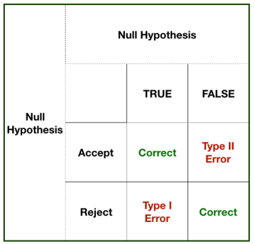
- Confidence Level: Probability of not making
- Type 1 Error: False positive, claiming something has happened when it has not
- Type ll Error: False negative, claiming something has not happened when it has
- Higher this value, larger test sample needed
- Common values: $0.90$ & $0.95$
Statistical Power:
Statistical Power: Probability of finding a statistically significant result when the Null Hypothesis is false
- Sample size increases = Power increases
- Confidence level increases = Power decreases
Connecting the Different Components
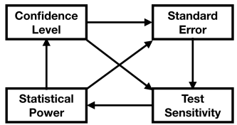
- Estimate our needed sample size from:
- needed level of sensitivity
- our desired test power & confidence level
Calculating the sample size and effect Size
To reach statistical significance, our sample size should be enough. To determine how many users we need for the test and control groups under various circumstances we will use the solve_power() function leaving nobs1 as None to get the needed sample size for our experiment.
Effect Size: The quantified magnitude of a result present in the population. Effect size is calculated using a specific statistical measure, such as Pearson’s correlation coefficient for the relationship between variables or Cohen’s d for the difference between groups.
from statsmodels.stats import power as pwr

# Calculate conversion rate mean and std
purchase_mean = df_merged.payment_confirm.mean()
purchase_std = df_merged.payment_confirm.std()

# Setting the parameters and we want to increase the purchase_mean to 0.1 in this experiment
effect_size = (0.1 - purchase_mean)/purchase_std
power = 0.8
alpha = 0.05

# Calculate ratio
sizes = [cont_n,test_n]
ratio = max(sizes)/min(sizes)

# Initialize analysis and calculate sample size
analysis = pwr.TTestIndPower()
ssresult = analysis.solve_power(effect_size=effect_size, power=power, alpha=alpha, nobs1=None, ratio=ratio)

print(f'Sample Size: {int(ssresult)}')
Effect Size
Knowing the needed sample size we calculate the minimum detectable effect size.
# Set parameters for entire dataset
alpha = 0.05
power = 0.8
samp_size = int(ssresult)

# Initialize analysis & calculate effect size
analysis = pwr.TTestIndPower()
esresult = analysis.solve_power(effect_size = None,
                                power = power,
                                nobs1 = samp_size,
                                ratio = ratio,
                                alpha = alpha)

print(f'Minimum detectable effect size: {round(esresult,2)}')
Statistical Power
Knowing the effect size and needed sample size we calculate Statistical Power.
# Set parameters
effect_size = esresult
alpha = 0.05

# Initialize analysis & calculate power
analysis = pwr.TTestIndPower()
pwresult = analysis.solve_power(effect_size=effect_size, power=None, alpha=alpha, nobs1=samp_size, ratio=ratio)

print(f'Power: {round(pwresult,3)}')
Analyzing the A/B test results
Confirming our test results
We will confirm that everything ran correctly for an A/B test. The checks we will perform will allow us to confidently report any results we uncover.
# Find the unique users in each group
results = df_merged.groupby('group').agg({'user_id': pd.Series.nunique})

# Find the overall number of unique users using "len" and "unique"
unique_users = len(df_merged.user_id.unique())

# Find the percentage in each group
results = results / unique_users * 100
print('Percentage of users in each group:','\n', results)
# Find the unique users in each group, by device and gender
results = df_merged.groupby(by=['group', 'device', 'sex']).agg({'user_id': pd.Series.nunique})

# Find the overall number of unique users using "len" and "unique"
unique_users = len(df_merged.user_id.unique())

# Find the percentage in each group
results = results / unique_users * 100
print('Percentage of users in each group:','\n', results)
Is the result statistically significant?
- Statistical Significance: Are the conversion rates different enough?
- If yes then we reject the null hypothesis
- Conclude that the paywall's have different effects
- If no then it may just be randomness
p-values
- probability if the Null Hypothesis is true...
- of observing a value as or more extreme than the one we observed
- Low p-values
- represent potentially significant results
- the observation is unlikely to have happened due to randomness
Interpreting p-values
- Controversial concept in some ways

Revisiting statistical significance
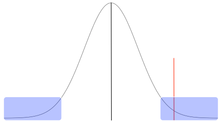
- Distribution of expected difference between control and test groups if the Null Hypothesis true
- Red line: The observed difference in conversion rates from our test
- p-value: Probability of being as or more extreme than the red line on either side of the distribution
Student's t-test
The t-test tells you how significant the differences between groups are; In other words it lets you know if those differences (measured in means or averages) could have happened by random chance.
Two basic types:
One-sample:Mean of population different from a given value?Two-sample:Two population means equal?
Checking for statistical significance l
Now that we have an intuitive understanding of statistical significance and p-values, we will apply it to our test result data.
Here we calculate the size of the test and control groups and calculate their respective conversion rates.
test = df_merged[df_merged.group == 'Test']
control = df_merged[df_merged.group == 'Control']

test_size = len(test['user_id'])
cont_size = len(control['user_id'])

cont_conv = control.payment_confirm.mean()
test_conv = test.payment_confirm.mean()

cont_conv_std = control.payment_confirm.std()
test_conv_std = test.payment_confirm.std()

print('Control Group Size:', cont_size)
print('Test Group Size:', test_size)

print(f'\nControl group conversion rate = {cont_conv}, std = {cont_conv_std}')
print(f'Test group conversion rate = {test_conv}, std = {test_conv_std}')
Checking for statistical significance ll
How we can certainly say this experiment is successful and the difference didn’t happen due to other factors?
To answer this question, we need to check if the uptick in the test group is statistically significant. scipy library allows us to programmatically check this with the stats.ttest_ind() function:
test_results = df_merged[df_merged.group == 'Test']['payment_confirm']
control_results = df_merged[df_merged.group == 'Control']['payment_confirm']

test_result = stats.ttest_ind(test_results, control_results)

statistic = test_result[0]
p_value = test_result[1]

print('statistic = ', statistic)
print('p_value = ', p_value)

# Check for statistical significance
if p_value >= 0.05:
    print("Not Significant")
else:
    print("Significant Result")
Sample Statistics versus Population
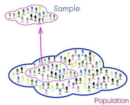
We will construct a sample by drawing points at random from the full dataset (population). We will compute the mean and standard deviation of the sample taken from that population to test whether the sample is representative of the population. Our goal is to see where the sample statistics are the same or very close to the population statistics.
subset_convs, test_sub_convs, cont_sub_convs = [], [], []
subset_convs_std, test_sub_convs_std, cont_sub_convs_std = [], [], []

for i in range(1000):
    subset = df_merged.sample(n=int(ssresult))

    test_sub = subset[subset.group == 'Test']
    control_sub = subset[subset.group == 'Control']

    subset_conv = subset.payment_confirm.mean()
    test_sub_conv = test_sub.payment_confirm.mean()
    control_sub_conv = control_sub.payment_confirm.mean()

    subset_conv_std = subset.payment_confirm.std()
    test_sub_conv_std = test_sub.payment_confirm.std()
    control_sub_conv_std = control_sub.payment_confirm.std()

    subset_convs.append(subset_conv)
    test_sub_convs.append(test_sub_conv)
    cont_sub_convs.append(control_sub_conv)

    subset_convs_std.append(subset_conv_std)
    test_sub_convs_std.append(test_sub_conv_std)
    cont_sub_convs_std.append(control_sub_conv_std)
Visualizing Variation of the samples
fig, ax = plt.subplots(nrows=1, ncols=3, figsize=(13,5))

ax[0].hist(subset_convs, bins=50, color='r', alpha=0.5, rwidth=0.75, label='Sample')
ax[1].hist(test_sub_convs, bins=50, color='b', alpha=0.5, rwidth=0.75, label='Test Sample')
ax[2].hist(cont_sub_convs, bins=50, color='g', alpha=0.5, rwidth=0.75, label='Control Sample')
ax[0].set_ylabel('Density', fontsize=14)
ax[0].set_title(f'Population sample mean = {round(np.mean(subset_convs),4)}, std = {round(np.mean(subset_convs_std),4)}', fontsize=12)
ax[1].set_title(f'Test sample mean = {round(np.mean(test_sub_convs),4)}, std = {round(np.mean(test_sub_convs_std),4)}', fontsize=12)
ax[2].set_title(f'Control sample mean = {round(np.mean(cont_sub_convs),4)}, std = {round(np.mean(cont_sub_convs_std),4)}', fontsize=12)
ax[0].legend()
ax[1].legend()
ax[2].legend()
plt.tight_layout()
fig.text(0.5, 0.001, 'Conversion Rate', ha='center', fontsize=14)
fig.suptitle(f'1k Random samples of conversion rate\'s', fontsize=24)
plt.subplots_adjust(top=.8)
plt.show()

print(f'Population: Conversion rate = {round(conversion_rate,4)}, Sample Conversion rate = {round(np.mean(subset_convs),4)}')
print(f'Control group: Population conversion rate = {round(cont_conv,4)}, Sample Conversion rate = {round(np.mean(cont_sub_convs),4)}')
print(f'Test group: Population conversion rate = {round(test_conv,4)}, Sample Conversion rate = {round(np.mean(test_sub_convs),4)}')

print(f'\nPopulation: Conversion std = {round(pop_std,4)}, Sample Conversion std = {round(np.mean(subset_convs_std),4)}')
print(f'Control group: Population conversion std = {round(cont_conv_std,4)}, Sample Conversion std = {round(np.mean(test_sub_convs_std),4)}')
print(f'Test group: Population conversion std = {round(test_conv_std,4)}, Sample Conversion std = {round(np.mean(cont_sub_convs_std),4)}')
What is a confidence interval
- Range of values for our estimation rather than single number
- Provides context for our estimation process
- Series of repeated experiments...
- the calculated intervals will contain the true parameter X% of the time
- The true conversion rate is a fixed quantity, our estimation and the interval are variable
Calculating confidence intervals
We will calculate the confidence intervals for the A/B test results.
def get_ci(value, cl, sd):
    loc = stats.norm.ppf(1 - cl/2)
    rng_val = stats.norm.cdf(loc - value/sd)

    lwr_bnd = value - rng_val
    upr_bnd = value + rng_val

    return_val = (lwr_bnd, upr_bnd)
    return(return_val)
# Calculate the mean of our lift distribution
lift_mean = test_conv - cont_conv

# Calculate variance and standard deviation
lift_variance = (1 - test_conv) * test_conv / test_size + (1 - cont_conv) * cont_conv / cont_size
lift_sd = lift_variance**0.5

# Find the confidence intervals with cl = 0.95
confidence_interval = get_ci(lift_mean, 0.95, lift_sd)
print('confidence_interval = ', confidence_interval)
Plotting the distribution
Here, we will visualize the test and control conversion rates as distributions. Additionally, viewing the data in this way can give a sense of the variability inherent in our estimation.
# Compute the variance
cont_var = (cont_conv * (1 - cont_conv)) / cont_size
test_var = (test_conv * (1 - test_conv)) / test_size

# Compute the standard deviations
control_sd = cont_var**0.5
test_sd = test_var**0.5

# Create the range of x values
control_line = np.linspace(cont_conv - 3 * control_sd, cont_conv + 3 * control_sd, 100)
test_line = np.linspace(test_conv - 3 * test_sd ,test_conv +  3 * test_sd, 100)

# Plot the distribution
plt.plot(control_line, stats.norm.pdf(control_line, cont_conv, control_sd), label='Test')
plt.plot(test_line, stats.norm.pdf(test_line, test_conv, test_sd), label='Control')
plt.legend()
plt.show()
Plotting the difference distribution
Now lets plot the difference distribution of our results that is, the distribution of our lift.
# Find the lift mean and standard deviation
sizes = [test_conv, cont_conv]
lift_mean = max(sizes) - min(sizes)
lift_sd = (test_var + cont_var) ** 0.5

# Generate the range of x-values
lift_line = np.linspace(lift_mean - 3 * lift_sd, lift_mean + 3 * lift_sd, 100)

# Find the confidence intervals with cl = 0.95
confidence_interval = get_ci(lift_mean, 0.95, lift_sd)

# Plot the lift distribution
plt.plot(lift_line, stats.norm.pdf(lift_line, lift_mean, lift_sd))

# Add the annotation lines
plt.axvline(x = lift_mean, color = 'r')
plt.title(f'Difference distribution confidence interval = {confidence_interval}')
plt.show()