Feature Extraction
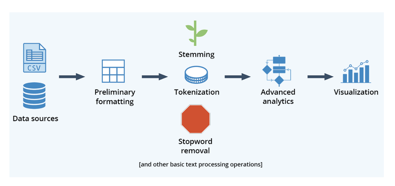
Feature extraction is the transformation of original data to a data set with a reduced number of variables, which contains the most discriminatory information. In a text or image classification problem, you have to extract features in order to train a model. These algorithms can interpret only numbers and you have to intelligently convert the text into the numerical feature vectors.

- Text classification or text categorization is an activity of labelling natural language texts with relevant predefined categories. The idea is to automatically organize text in different classes.
If you think about it, text is just a series of ordered words that usually carry some meaning. If we take each unique word from all the available texts, we can create our own vocabulary. And every word in the vocabulary can be a feature. For each text a feature vector will be an array where feature values are simply the numbers of the unique words belonging to a specific text, i.e. just the count of each word in one text. And if some word is not in the text, its feature value is zero. Therefore, the word order in a text is not important, just the number of occurrences. This method is called a Bag of words BOW and it’s quite common and simple to use.
- To solve the problem of word order we use another approach called Word Embedding.
- Word Embedding: It is a representation of text where words that have the same meaning have a similar representation. In other words it represents words in a coordinate system where related words, based on a corpus of relationships, are placed closer together.
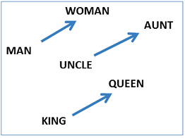
- Word2vec is a model of word embedding that takes as input a large corpus of text and produces a vector space with each unique word being assigned a corresponding vector in the space. Word vectors are positioned in the vector space such that words that share common contexts in the corpus are located in close proximity to one another in the space. Word2Vec is very famous at capturing meaning and demonstrating it on tasks like calculating analogy questions of the form a is to b as c is to ?. For example, man is to woman as uncle is to ? (aunt) using a simple vector offset method based on
cosine distance. For example, here are vector offsets for three word pairs illustrating the gender relation:


A tf-idf word-frequency array
tf–idforTFIDF, short forterm frequency–inverse document frequency, is a numerical statistic that is intended to reflect how important a word is to a document in a collection or corpus. It is often used as a weighting factor in searches of information retrieval, text mining, and user modeling. Thetf–idfvalue increases proportionally to the number of times a word appears in the document and is offset by the number of documents in the corpus that contain the word, which helps to adjust for the fact that some words appear more frequently in general.tf–idfis one of the most popular term-weighting schemes today;83% of text-based recommender systems in digital libraries use tf–idf.

In this exercise, we create a tf-idf word frequency array for a toy collection of documents. For this, use the TfidfVectorizer from sklearn. It transforms a list of documents into a word frequency array, which it outputs as a csr_matrix. It has fit() and transform() methods like other sklearn objects.
TruncatedSVD and csr_matrix
TruncatedSVD singular value decomposition (SVD) is able to perform PCA on sparse arrays in csr_matrix format, such as word-frequency arrays.
- scikit-learn PCA doesn't support
csr_matrix - Use scikit-learn
TruncatedSVDinstead - Performs same transformation
import warnings
warnings.filterwarnings('ignore')
from sklearn.decomposition import TruncatedSVD
from sklearn.feature_extraction.text import TfidfVectorizer

documents = ['cats say meow', 'dogs say woof', 'dogs chase cats', 'never say ever',
            'faith for one', 'faith to one', 'i hate dogs', 'i hate cats']

model = TruncatedSVD(n_components=8)

# Create a TfidfVectorizer: tfidf
tfidf = TfidfVectorizer()

# Apply fit_transform to document: csr_mat
csr_mat = tfidf.fit_transform(documents)
print(csr_mat.toarray())

model.fit(csr_mat)
transformed = model.transform(csr_mat)

# Get the words: words
words = tfidf.get_feature_names()

# Print words
print('\n',words)
import matplotlib.pyplot as plt
import seaborn as sns
import numpy as np

var_ratio = model.explained_variance_ratio_
cum_var_ratio = np.cumsum(var_ratio)
col_num = model.n_components
feat_names = ['C'+str(num) for num in list(range(1,col_num+1,1))]

sns.barplot(y=var_ratio, x=feat_names)
sns.pointplot(y=var_ratio, x=feat_names, color='black')
plt.grid(False)
plt.title("Explained variance Ratio by each component", fontsize=14)
plt.ylabel("Explained variance ratio (%)")
plt.show()
DictVectorizer
- The class DictVectorizer can be used to convert feature arrays represented as lists of standard Python dict objects to the NumPy/SciPy representation used by scikit-learn estimators.
- DictVectorizer implements what is called one-of-K or “
one-hot” coding for categorical (aka nominal, discrete) features.
from sklearn.feature_extraction import DictVectorizer

v = DictVectorizer(sparse=False)

d = [{'height': 1, 'length': 0, 'width': 1},
     {'height': 2, 'length': 1, 'width': 0},
     {'height': 1, 'length': 3, 'width': 2}]

v.fit_transform(d)
v.get_feature_names()
DictVectorizer is also a useful representation transformation for training sequence classifiers in Natural Language Processing models that typically work by extracting feature windows around a particular word of interest.
- For example, suppose that we have a first algorithm that extracts Part of Speech (PoS) tags that we want to use as complementary tags for training a sequence classifier (e.g. a chunker). The following dict could be such a window of features extracted around the word ‘
sat’ in the sentence ‘The cat sat on the mat.’:
pos_window = [
        {
         'word-2': 'the',
         'pos-2': 'DT',
         'word-1': 'cat',
         'pos-1': 'NN',
         'word+1': 'on',
         'pos+1': 'PP',
     },
    ]
This description can be vectorized into a sparse two-dimensional matrix suitable for feeding into a classifier
vec = DictVectorizer()
pos_vectorized = vec.fit_transform(pos_window)
pos_vectorized.toarray()
vec.get_feature_names()
Note that this transformer will only do a binary one-hot encoding when feature values are of type string.
20 newsgroups dataset
The 20 newsgroups dataset comprises around 18000 newsgroups posts on 20 topics split in two subsets: one for training (or development) and the other one for testing (or for performance evaluation). The split between the train and test set is based upon a messages posted before and after a specific date.
from sklearn import datasets

news = datasets.fetch_20newsgroups(subset='all')

X = news.data
y = news.target
print("Number of articles: " + str(len(X)))
print("Number of diffrent categories: " + str(len(news.target_names)))
news.target_names
import pandas as pd

df = pd.DataFrame({'class': y,
                   'text':  X })
df
df.text[0]
To get the frequency distribution of the words in the text, we can utilize the nltk.FreqDist() function, which lists the top words used in the text, providing a rough idea of the main topic in the text data:
reviews = df.text.str.cat(sep=' ')

#function to split text into word
tokens = word_tokenize(reviews)

vocabulary = set(tokens)

print(len(vocabulary))

frequency_dist = nltk.FreqDist(tokens)

print(sorted(frequency_dist,key=frequency_dist.__getitem__, reverse=True)[0:50])
This gives the top 50 words used in the text, though it is obvious that some of the stop words, such as the, frequently occur in the English.
Let us remove punctuation to further cleanup the text corpus.
import string

punc = list(string.punctuation)
tokens = [w for w in tokens if not w in punc]
print(tokens[0:50])
stop words
Stop words are words that don’t bring any useful information in the processing text and they are usually filtered out before or after processing. They refer to the most common words like I, her, by, about, here, etc. Removing such words in the context of sentiment analysis can easily upgrade your accuracy significantly.
from nltk.corpus import stopwords

stop_words = set(stopwords.words('english'))
tokens = [w for w in tokens if not w in stop_words]
print(tokens[0:50])
A helpful visualization tool wordcloud helps to create word clouds by placing words on a canvas randomly, with sizes proportional to their frequency in the text.
from wordcloud import WordCloud
import matplotlib.pyplot as plt

frequency_dist = nltk.FreqDist(tokens)
wordcloud = WordCloud().generate_from_frequencies(frequency_dist)

plt.figure(figsize=(12,8))
plt.imshow(wordcloud)
plt.axis("off")
plt.show()
Plot count of individual class occurrences
f, axe = plt.subplots(1, 1,figsize=(14,5))
axe.grid(False)
sns.despine(left=True, bottom=True)
sns.countplot(df['class'], ax=axe)
for p in axe.patches:
        axe.annotate('{}'.format(p.get_height()), (p.get_x()+0.15, p.get_height()+30),
                     color='k', fontweight='medium', fontsize=12)
        axe.yaxis.tick_left()
        axe.set_xlabel('Target', fontsize=14)
        axe.set_ylabel('Number of Occurrences', fontsize=14)
there are 18846 newsgroup documents, distributed almost evenly across 20 different newsgroups. Our goal is to create a classifier that will classify each document based on its content.
Define training function
from sklearn.model_selection import train_test_split
import time

def train(classifier, X, y):
    start = time.time()
    X_train, X_test, y_train, y_test = train_test_split(X, y, test_size=0.2, random_state=11)

    classifier.fit(X_train, y_train)
    end = time.time()

    print("Accuracy: " + str(classifier.score(X_test, y_test)) + ", Training Duration: " + str(end - start))
- let’s build a classifier! We’ll start with a multinomial Naive Bayes classifier which is suitable for discrete classification.
- The
multinomial Naive Bayesclassifier is suitable for classification with discrete features (e.g., word counts for text classification). The multinomial distribution normally requires integer feature counts. However, in practice, fractional counts such as tf-idf may also work.
- The multinomial distribution is a generalization of the binomial distribution. For example, it models the probability of counts for each side of a k-sided die rolled n times. For n independent trials each of which leads to a success for exactly one of k categories, with each category having a given fixed success probability, the multinomial distribution gives the probability of any particular combination of numbers of successes for each categories.
from sklearn.naive_bayes import MultinomialNB
from sklearn.pipeline import Pipeline
from sklearn.feature_extraction.text import TfidfVectorizer

trial1 = Pipeline([ ('vectorizer', TfidfVectorizer()), ('classifier', MultinomialNB())])

train(trial1, X, y)
Let us remove the stop words to further cleanup the text corpus.
from nltk.corpus import stopwords

trial2 = Pipeline([ ('vectorizer', TfidfVectorizer(stop_words=stopwords.words('english'))),
                   ('classifier', MultinomialNB())])

train(trial2, X, y)
Parameter tuning
Accuracy is better and the training is faster, but the alpha parameter of the Naive-Bayes classifier is the default, so let’s do some hyperparameter tuning.
- We will use
GridSearchCVan exhaustive search over specified parameter values for an estimator.
# Find correct parameter name for the estimator
trial2.get_params().keys()
from sklearn.model_selection import GridSearchCV

# Number of cross validation folds
n_folds = 5

# Returns a range between two values evenly sampled in log space.
alpha = np.geomspace(0.05, 0.00005, 30)

param_grid1 = {'classifier__alpha': alpha}

estimator1 = GridSearchCV(estimator=trial2,
                         param_grid=param_grid1,
                         n_jobs=4,
                         cv=n_folds,
                         return_train_score=True,
                         scoring='accuracy'
                        )

estimator1.fit(X=X, y=y)
Create df of search results to plot
results1 = estimator1.cv_results_

test_scores1 = pd.DataFrame({fold: results1[f'split{fold}_test_score'] for fold in range(n_folds)},
                           index=alpha).stack().reset_index()

test_scores1.columns = ['alpha', 'fold', 'accuracy']
mean1 = test_scores1.groupby('alpha').accuracy.mean()
best_alpha1, best_score1 = mean1.idxmin(), mean1.min()
test_scores1.head()
Function to plot grid search
def plot_results(model, name='Num Trees', param_name = 'param_regressor__min_samples_split'):
    # param_name = param_name
    # Extract information from the cross validation model
    train_scores = model.cv_results_['mean_train_score']
    test_scores = model.cv_results_['mean_test_score']
    train_time = model.cv_results_['mean_fit_time']
    param_values = list(model.cv_results_[param_name])

    # Plot the scores over the parameter
    plt.subplots(1, 2, figsize=(14, 5))
    plt.subplot(121)
    plt.errorbar(param_values, train_scores, yerr=train_scores.std(), label = 'train', color='b', fmt='-o')
    plt.errorbar(param_values, test_scores, yerr=test_scores.std(), label = 'test', color='red', fmt='-o')
    plt.legend(bbox_to_anchor=(1, 1.05), prop={'size': 14})
    plt.grid(False)
    plt.xlabel(name, fontsize=14)
    plt.ylabel('Accuracy', fontsize=14)
    plt.title(f'Score vs {name}', fontsize=14)

    plt.subplot(122)
    plt.plot(param_values, train_time, 'ro-', color='y')
    plt.xlabel(name, fontsize=14)
    plt.ylabel('Train Time (sec)', fontsize=14)
    plt.title('Training Time vs %s' % name, fontsize=14)
    plt.grid(False)
    plt.tight_layout(pad = 1)
    plt.show();
estimator1.cv_results_.keys()
print(f'GridSearchCV Results Best Alpha: {best_alpha1} | Best Accuracy: {best_score1:.3f}')

plot_results(estimator1, name = 'Alpha',
             param_name='param_classifier__alpha')
We can see that the best accuracy for alpha found by GridSearchCV is an improvement now lets set the parameter min_dif to ignore the words that appear fewer than x times in all documents:
for min_df in [0, 2, 3, 4, 5]:
    trial3 = Pipeline([('vectorizer', TfidfVectorizer(stop_words=stopwords.words('english'),
                                                      min_df=min_df)),
                       ('classifier', MultinomialNB(alpha=best_alpha1))])

    print(f'\nTraining min_df = {min_df}')
    train(trial3, X, y)
Resulting accuracy slightly decreased. We can try and stem the data with nltk (i.e. reduce inflected words to their word root, with he use of tokenizer within TfidfVectorizer, it usually helps performance, and we can add punctuations to a list of stop words nltks string.

- Stemming is a process of reducing inflected words to their word stem, i.e root. It doesn’t have to be morphological; you can just chop off the words ends. For example, the word “solv” is the stem of words “solve” and “solved”.
- Lemmatization is another approach to remove inflection by determining the part of speech and utilizing detailed database of the language.
- The lemmatized form of studies is: study
- The lemmatized form of studying is: study
- Tokenization converts sentences to words.
# using NLTK library, we can do lot of text preprocesing
import nltk
from nltk.tokenize import word_tokenize

#function to split text into word
tokens = word_tokenize("The quick brown fox jumps over the lazy dog")
print(tokens)
# NLTK provides several stemmer interfaces like Porter stemmer, #Lancaster Stemmer, Snowball Stemmer
from nltk.stem import PorterStemmer

porter = PorterStemmer()
stems = []
for t in tokens:
    stems.append(porter.stem(t))
print(stems)
import string

def stemming_tokenizer(text):
    stemmer = PorterStemmer()
    return [stemmer.stem(w) for w in word_tokenize(text)]

trial5 = Pipeline([ ('vectorizer', TfidfVectorizer(tokenizer=stemming_tokenizer,
                     stop_words=stopwords.words('english') + list(string.punctuation))),
                    ('classifier', MultinomialNB(alpha=0.005))])

train(trial5, X, y)
Accuracy is slightly better, but the training was much longer. This is a great example of time consumption created by stemming. Sometimes accuracy can cost you computation speed and you should find a balance between the two. Don’t stem if the accuracy doesn’t improve significantly.
Test different classifiers
Now, let’s try some other usual text classifiers like Support Vector Classification with stochastic gradient descent SGDClassifier and linear SVC. They are initially slower but may get better accuracy without the use of a stemmer:
from sklearn.linear_model import SGDClassifier
from sklearn.svm import LinearSVC
from sklearn.ensemble import RandomForestClassifier

for classifier in [SGDClassifier(), LinearSVC()]:

    trial6 = Pipeline([('vectorizer', TfidfVectorizer(stop_words=stopwords.words('english') + list(string.punctuation))),
                       ('classifier', classifier)])

    print(f'\nTraining with {classifier.__class__.__name__}')
    train(trial6, X, y)
An accuracy of 93.2% for linear SVC is very acceptable. Acceptable accuracy depends on the specific problem: type/length of the text, number of categories and differences between them, etc. Here, an accuracy of 93% is good because we have 20 categories and some of them are similar, like comp.sys.ibm.pc.hardware and comp.sys.mac.hardware.
Model evaluation
We could diver deeper but we will stop here and check the characteristics of the best model. We will use confusion_matrix() from sckit-learn to compare real and predicted categories:
from sklearn.metrics import confusion_matrix
import matplotlib.pyplot as plt

start = time.time()
classifier = Pipeline([('vectorizer', TfidfVectorizer(stop_words=stopwords.words('english') + list(string.punctuation))),
                       ('classifier', LinearSVC(C=10))])

X_train, X_test, y_train, y_test = train_test_split(news.data, news.target,
                                                    test_size=0.2, random_state=11)
classifier.fit(X_train, y_train)
end = time.time()

print("Accuracy: " + str(classifier.score(X_test, y_test)) + ", Time duration: " + str(end - start))
y_pred = classifier.predict(X_test)
conf_mat = confusion_matrix(y_test, y_pred)
labels = news.target_names

# Plot confusion_matrix
fig, ax = plt.subplots(figsize=(13, 10))
sns.heatmap(conf_mat, annot=True, fmt ="d", cmap = "Set3",
xticklabels=labels, yticklabels=labels)
plt.ylabel('Actual', fontsize=14)
plt.xlabel('Predicted', fontsize=14)
b, t = plt.ylim()
b += 0.5
t -= 0.5
plt.ylim(b, t)
plt.show()
The confusion matrix is a great way to see which categories the model is mixing. For example, there are 17 articles from category comp.os.ms-windows.mics that are wrongly classified as comp.sys.ibm.pc.hardware. Also, let’s check the accuracy of each category separately with classification_report():
from sklearn import metrics
print(metrics.classification_report(y_test, y_pred, target_names=labels))
Category misc.forsale has the lowest accuracy, but the overall accuracy is good.
Finally lets take a look at the PrecisionRecallCurve and not the most ideal in this situation but for kicks the ROC curve.
from yellowbrick.classifier import PrecisionRecallCurve
from yellowbrick.classifier import ROCAUC

fig, ax = plt.subplots(figsize=(10, 5))
roc = ROCAUC(classifier, classes=labels, ax=ax)
roc.fit(X_train, y_train)
roc.score(X_test, y_test)
plt.title('ROC AUC', fontweight='bold', fontsize=14)
plt.xlabel('False Positive Rate', fontsize=14)
plt.ylabel('True Positive Rate', fontsize=14)
plt.grid(False)
plt.legend(bbox_to_anchor=(1.1, 1.05))
plt.show();

fig, ax = plt.subplots(figsize=(10, 5))
prc = PrecisionRecallCurve(classifier, ax=ax)
prc.fit(X_train, y_train)
prc.score(X_test, y_test)
plt.title('Precision Recall Curve', fontweight='bold', fontsize=14)
plt.xlabel('Recall', fontsize=14)
plt.ylabel('Precision', fontsize=14)
plt.grid(False)
plt.legend()
plt.show();