What is machine learning?

The art and science of: Giving computers the ability to learn to make decisions from data without being explicitly programmed!

The machine learning workflow

• The following chart outlines the key steps from problem definition to the deployment of a predictive solution:

• The process is iterative throughout the sequence, and the effort required at different stages will vary according to the project, but this process should generally include the following steps:

  1. Frame the problem, identify a target metric, and define success
  2. Source, clean, and validate the data
  3. Understand your data and generate informative features
  4. Pick one or more machine learning algorithms suitable for your data
  5. Train, test, and tune your models
  6. Use your model to solve the original problem

Naming conventions

• Features or predictor variables or independent variables
• Target variable or dependent variable or response variable

• Examples:
  • Learning to predict whether an email is spam or not
  • Clustering wikipedia entries into different categories
  • Supervised learning: Uses labeled data
  • Unsupervised learning: Uses unlabeled data

• The key challenge of automated learning is to identify patterns in the training data that are meaningful when generalizing the model's learning to new data. There are a large number of potential patterns that a model could identify, while the training data only constitute a sample of the larger set of phenomena that the algorithm needs to predict in the future.

• A learner's hypothesis space has to be tailored to a specific task using prior knowledge about the task domain in order for the search of meaningful patterns to succeed. We must pay close attention to the assumptions that a model makes about data relationships for a specific task and emphasize the importance of matching these assumptions with empirical evidence gleaned from data exploration.

Supervised learning

• Predictor variables + a labeled target variable

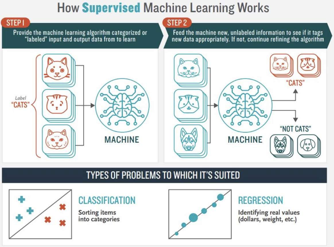
• The term supervised implies the presence of an outcome variable that guides the learning process—that is, it teaches the algorithm the correct solution to the task that is being learned.

Unsupervised learning

• Uncovering hidden patterns from unlabeled data

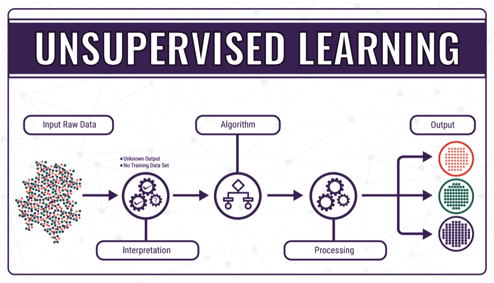
• When solving an unsupervised learning problem, we only observe the features and have no measurements of the outcome. Instead of the prediction of future outcomes or the inference of relationships among variables. The task is to find structure in the data without any outcome information to guide the search process.

• Often, unsupervised algorithms aim to learn a new representation of the input data that is useful for some other tasks. This includes coming up with labels that identify commonalities among observations, or a summarized description that captures relevant information while requiring data points or features.

• Examples:
  • Grouping customers into distinct categories
  • Anomaly Detection
  • Document Classification
  • Grouping together securities with similar risk and return characteristics
  • Finding a small number of risk factors driving the performance of a much larger number of securities

Cluster algorithms

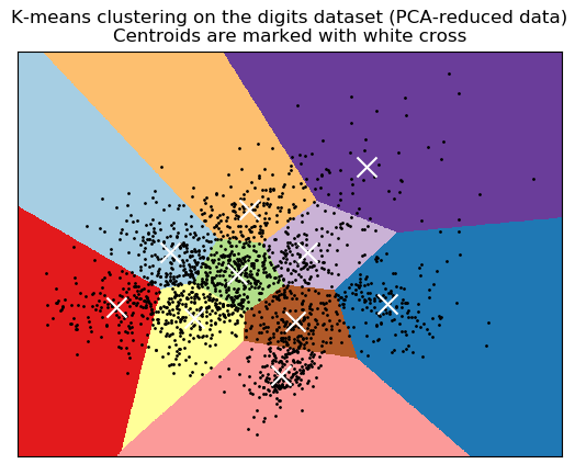
• Cluster algorithms use a measure of similarity to identify observations or data attributes that contain similar information. They summarize a dataset by assigning a large number of data points to a smaller number of clusters so that the cluster members are more closely related to each other than to members of other clusters.

• Cluster algorithms primarily differ with respect to the type of clusters that they will produce, which implies different assumptions about the data generation process, listed as follows:

• K-means clustering: Data points belong to one of the k clusters of equal size that take an elliptical form

• Gaussian mixture models: Data points have been generated by any of the various multivariate normal distributions

• Density-based clusters: Clusters are of an arbitrary shape and are defined only by the existence of a minimum number of nearby data points

• Hierarchical/Agglomerative clusters: Data points belong to various supersets of groups that are formed by successively merging into smaller clusters based on a linkage criteria (criteria for calculating the distance between the newly formed cluster).

Dimensionality reduction & feature selection

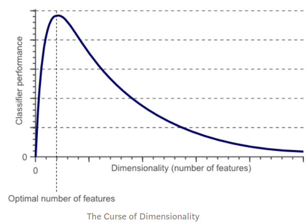
• As the number of features increases, the model becomes more complex. Having more features increases the likelihood of overfitting. A machine learning model that is trained on a large number of features, gets increasingly dependent on the training data and in turn could overfit, resulting in poor performance on new data.

• Dimensionality reduction produces new data that captures the most important information contained in the source data. Rather than grouping existing data into clusters, these algorithms transform existing data into a new dataset that uses significantly fewer features or observations to represent the original information.

Linear Dimensionality Reduction:

• Factor Analysis: Used to reduce a large number of variables into a fewer numbers of factors. The values of observed data are expressed as functions of a number of possible causes in order to find which are the most important. The observations are assumed to be caused by a linear transformation of lower dimensional latent factors and added Gaussian noise.

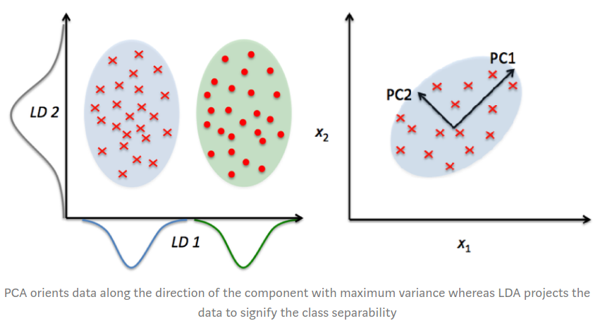
• Principal component analysis (PCA): Finds the linear transformation that captures most of the variance in the existing dataset. PCA Algorithms differ with respect to the nature of the new dataset they will produce.

• LDA (Linear Discriminant Analysis) projects data in a way that the class separability is maximised. Examples from same class are put closely together by the projection. Examples from different classes are placed far apart by the projection
  • LDA makes some simplifying assumptions about your data: That your data is Gaussian, that each variable is is shaped like a bell curve when plotted.
  • That each attribute has similar variance, that values of each variable vary around the mean by the same amount on average.

• Extensions to LDA:

  • Quadratic Discriminant Analysis (QDA): Each class uses its own estimate of variance (or covariance when there are multiple input variables).

  • Flexible Discriminant Analysis (FDA): Where non-linear combinations of inputs are used such as splines.

  • Regularized Discriminant Analysis (RDA): Introduces regularization into the estimate of the variance (actually covariance), moderating the influence of different variables on LDA.

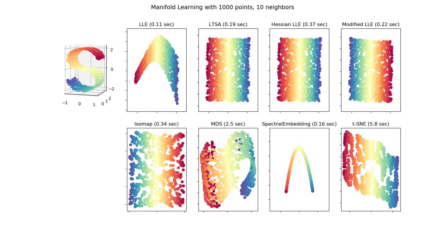
Non-linear Dimensionality Reduction Methods (Manifold learning):

• Identifies a nonlinear transformation that produces a lower-dimensional representation of the data.

• Multi-dimensional scaling (MDS) : A technique used for analyzing similarity or dissimilarity of data as distances in a geometric spaces. Projects data to a lower dimension such that data points that are close to each other (in terms if Euclidean distance) in the higher dimension are close in the lower dimension as well.

• Isometric Feature Mapping (Isomap) : Projects data to a lower dimension while preserving the geodesic distance (rather than Euclidean distance as in MDS). Geodesic distance is the shortest distance between two points on a curve.

• Locally Linear Embedding (LLE): Recovers global non-linear structure from linear fits. Each local patch of the manifold can be written as a linear, weighted sum of its neighbours given enough data.

• Hessian Eigenmapping (HLLE): Projects data to a lower dimension while preserving the local neighbourhood like LLE but uses the Hessian operator to better achieve this result and hence the name.

• Spectral Embedding (Laplacian Eigenmaps): Uses spectral techniques to perform dimensionality reduction by mapping nearby inputs to nearby outputs. It preserves locality rather than local linearity

• t-distributed Stochastic Neighbor Embedding (t-SNE): Computes the probability that pairs of data points in the high-dimensional space are related and then chooses a low-dimensional embedding which produce a similar distribution.

• Autoencoders: Uses neural networks to compress data non-linearly with minimal loss of information.

Null Hypothesis and Testing

• A null hypothesis, proposes that no significant difference exists in a set of observations.

• Null: The two sample means are equal

• Alternate: The two sample means are not equal

• For rejecting a null hypothesis, a test statistic is calculated. This test-statistic is then compared with a critical value and if it is found to be greater than the critical value the hypothesis is rejected.

• Hypothesis tests are based on the notion of critical regions: the null hypothesis is rejected if the test statistic falls in the critical region. The critical values are the boundaries of the critical region. If the test is one-sided (like a χ2 test or a one-sided t-test) then there will be just one critical value, but in other cases (like a two-sided t-test) there will be two.

What is a critical value?

• In hypothesis testing, a critical value is a point on the test distribution that is compared to the test statistic to determine whether to reject the null hypothesis. If the absolute value of your test statistic is greater than the critical value, you can declare statistical significance and reject the null hypothesis. Critical values correspond to α or alpha (constant), so their values become fixed when you choose the test's α.

Critical values on the standard normal distribution for α = 0.05

• Figure A shows that results of a one-tailed Z-test are significant if the test statistic is equal to or greater than 1.64, the critical value in this case. The shaded area is 5% (α) of the area under the curve.

• Figure B shows that results of a two-tailed Z-test are significant if the absolute value of the test statistic is equal to or greater than 1.96, the critical value in this case. The two shaded areas sum to 5% (α) of the area under the curve.

Z-test

• In a z-test, the sample is assumed to be normally distributed. A z-score is calculated with population parameters such as “population mean” and “population standard deviation” and is used to validate a hypothesis that the sample drawn belongs to the same population.

• The hypothesis being tested for z-test is:
  • Null: Sample mean is same as the population mean
  • Alternate: Sample mean is not same as the population mean

• The statistics used for this hypothesis testing is called z-statistic. If the test statistic is lower than the critical value, accept the hypothesis or else reject the hypothesis

T-test

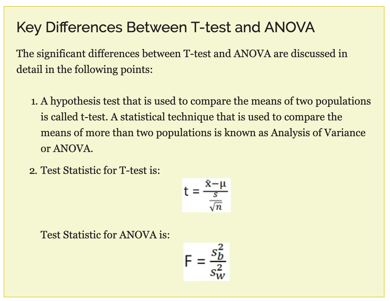
• A t-test is used to compare the mean of two given samples. Like a z-test, a t-test also assumes a normal distribution of the sample. A t-test is used when the population parameters (mean and standard deviation) are not known.

• Three versions of t-test:
  1. Independent samples t-test which compares mean for two groups
  2. Paired sample t-test which compares means from the same group at different times
  3. One sample t-test which tests the mean of a single group against a known mean.

Univariate Feature Selection:

• Univariate Feature Selection uses statistical tests to select features. Univariate consists of observations on only a single characteristic or attribute. Univariate feature selection examines each feature individually to determine the strength of the relationship of the feature with the response variable.

• Some examples of statistical tests that can be used to evaluate feature relevance are: Pearson Correlation, Maximal information coefficient, Distance correlation, ANOVA and Chi-square.

• Scikit-learn exposes feature selection routines likes SelectKBest, SelectPercentile or GenericUnivariateSelect as objects that implement a transform method based on the score of anova or chi2, mutual information or fpr/fdr,fwe (false positive rate, false discovery rate, family-wise error rate).

Chi-square:

• Used to find the relationship between categorical variables. The chi-square test of independence works by comparing the categorically coded data that you have collected (known as the observed frequencies) with the frequencies that you would expect to get in each cell of a contingency table by chance alone (known as the expected frequencies).

Two types of chi-square test

1. Goodness of fit test, which determines if a sample matches the population.

1. A chi-square fit test for two independent variables is used to compare two variables in a contingency table to check if the data fits.

   • small chi-square value means that data fits.
   • high chi-square value means that data doesn’t fit.

• The hypothesis being tested for chi-square is:
  • Null: Variable A and Variable B are independent
  • Alternate: Variable A and Variable B are not independent.

Anova:

• Analysis of variance is preferred when the variables are continuous. Analysis of variance (ANOVA) is an analysis tool used in statistics that splits an observed aggregate variability found inside a data set into two parts: systematic factors and random factors. The systematic factors have a statistical influence on the given data set, while the random factors do not.

• The hypothesis being tested for anova is:
  • Null: All pairs of samples are same i.e. all sample means are equal
  • Alternate: At least one pair of samples is significantly different

Mutual Information:

• The mutual information (MI) between a feature and the outcome is a measure of the mutual dependence between the two variables. It extends the notion of correlation to nonlinear relationships. More specifically, it quantifies the information obtained about one random variable through the other random variable. The concept of MI is closely related to the fundamental notion of entropy of a random variable. Entropy quantifies the amount of information contained in a random variable.

• For regression: f_regression (anova), mutual_info_regression

• For classification: chi2, f_classif (anova), mutual_info_classif
  • F-Test checks for and only captures linear relationships between features and labels. A highly correlated feature is given higher score and less correlated features are given lower score.

Deep learning and AI

• Artificial intelligence (AI) refers to the simulation of human intelligence in machines that are programmed to think like humans and mimic their actions. The term may also be applied to any machine that exhibits traits associated with a human mind such as learning and problem-solving. The ideal characteristic of artificial intelligence is its ability to rationalize and take actions that have the best chance of achieving a specific goal.

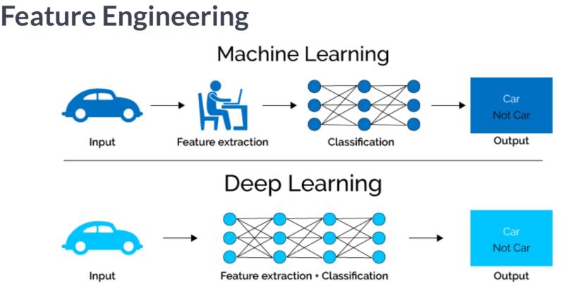
• Deep learning is an artificial intelligence function that imitates the workings of the human brain in processing data and creating patterns for use in decision making. Deep learning is a subset of machine learning in artificial intelligence (AI) that has networks capable of learning unsupervised from data that is unstructured or unlabeled. Also known as deep neural learning or deep neural network.

• A Neural Network is a series of algorithms that endeavors to recognize underlying relationships in a set of data through a process that mimics the way the human brain operates. In this sense, neural networks refer to systems of neurons, either organic or artificial in nature. Neural networks can adapt to changing input; so the network generates the best possible result without needing to redesign the output criteria.

Reinforcement learning

• Software agents interact with an environment

• Learn to choose the action that yields the highest reward, given a set of input data that describes a context or environment. It is both dynamic and interactive: the stream of positive and negative rewards impacts the algorithm's learning, and actions taken now may influence both the environment and future rewards.

• Draws inspiration from behavioral psychology

• Reinforcement learning differs from supervised learning, where the available training data lays out both the context and the correct decision for the algorithm. It is tailored to interactive settings where the outcomes only become available over time and learning has to proceed in an online or continuous fashion as the agent acquires new experience.

The trade-off

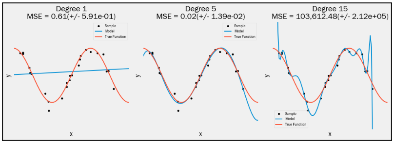
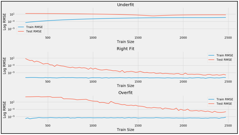
• More complex models have more moving parts that are capable of representing more nuanced relationships, but they may also be more difficult to inspect. They are also likely to overfit and learn random noise particular to the training sample, as opposed to a systematic signal that represents a general pattern of the input- output relationship. Overly simple models, on the other hand, will miss signals and deliver biased results. This trade-off is known as the bias-variance trade-off

Regression problems

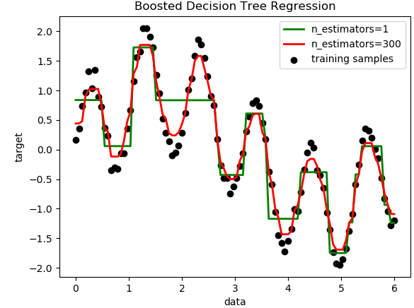
• Regression problems aim to predict a continuous variable. The root-mean-square error (RMSE) is the most popular loss function and error metric. The loss is symmetric, but larger errors weigh more in the calculation. Using the square root has the advantage of measuring the error in the units of the target variable.

• The explained variance score computes the proportion of the target variance that the model accounts for and varies between 0 and 1. The R2 score or coefficient of determination yields the same outcome the mean of the residuals is 0, but can differ otherwise.

Classification problems

• Classification problems have categorical outcome variables. Most predictors will output a score to indicate whether an observation belongs to a certain class. In the second step, these scores are then translated into actual predictions.

• Binary classification problem: A classification task with only two classes; e.g., learning to predict whether an email is spam or not. In the binary case, where we will label the classes positive and negative, the score typically varies between zero or is normalized accordingly. Once the scores are converted into 0-1 predictions, there can be four outcomes, because each of the two existing classes can be either correctly or incorrectly predicted. With more than two classes, there can be more cases if you differentiate between the several potential mistakes.

• Multiclass classification problem: A classification task with more than two classes; e.g., classify a set of images of fruits which may be oranges, apples, or pears. Multi-class classification makes the assumption that each sample is assigned to one and only one label: a fruit can be either an apple or a pear but not both at the same time.

Classification metrics

Measuring model performance

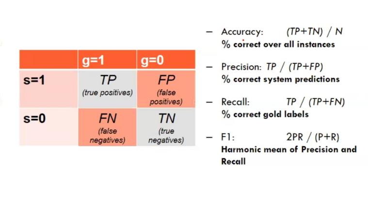
• High precision: Not many real emails predicted as spam
• High recall: Predicted most spam emails correctly

Receiver operating characteristics and the area under the curve

• The receiver operating characteristics (ROC) curve allows us to visualize, organize, and select classifiers based on their performance. It computes all the combinations of true positive rates (TPR) and false positive rates (FPR) that result from producing predictions using any of the predicted scores as a threshold. It then plots these pairs on a square, the side of which has a measurement of one in length.

• The area under the curve (AUC) is defined as the area under the ROC plot that varies between 0.5 and the maximum of 1. It is a summary measure of how well the classifier's scores are able to rank data points with respect to their class membership. More specifically, the AUC of a classifier has the important statistical property of representing the probability that the classifier will rank a randomly chosen positive instance higher than a randomly chosen negative instance, which is equivalent to the Wilcoxon ranking test. In addition, the AUC has the benefit of not being sensitive to class imbalances.

Precision-recall curves

When predictions for one of the classes are of particular interest, precision and recall curves visualize the trade-off between these error metrics for different thresholds. Both measures evaluate the quality of predictions for a particular class. The following list shows how they are applied to the positive class:

• Classification Accuracy is simply the rate of correct classifications
• Recall measures the share of actual positive class members that a classifier predicts as positive for a given threshold.
• Precision, in contrast, measures the share of positive predictions that are correct.

• Recall typically increases with a lower threshold, but precision may decrease. Precision-recall curves visualize the attainable combinations and allow for the optimization of the threshold given the costs and benefits of missing a lot of relevant cases or producing lower-quality predictions.

• The F1 score is a harmonic mean of precision and recall for a given threshold and can be used to numerically optimize the threshold while taking into account the relative weights that these two metrics should assume.

Class imbalance

Imbalanced Datasets:

• Never test on the oversampled or undersampled dataset.
• If we want to implement cross validation, remember to oversample or undersample your training data during cross-validation, not before!
• Don't use accuracy score as a performance metric with imbalanced datasets (will be usually high and misleading). You could build a classifier that predicts ALL emails as real and be 99% accurate! But horrible at actually classifying emails as spam. Therefore failing at its original purpose. Instead use f1-score, precision/recall score or confusion matrix.

Class imbalance example:

• 99% of emails are real; 1% of emails are spam

• To improve the performance of imbalanced datasets
  • Under-sampling: Remove samples from over-represented classes ; use this if you have huge dataset
  • Over-sampling: Add more samples from under-represented classes; use this if you have small dataset

• Despite the advantage of balancing classes, these techniques also have their weaknesses. The simplest implementation of over-sampling is to duplicate random records from the minority class, which can cause overfitting. In under-sampling, the simplest technique involves removing random records from the majority class, which can cause loss of information.

• Sub-Sampling: A method of Under-sampling, for example a dataframe with a 50/50 ratio of real and spam-emails. Meaning our sub-sample will have the same amount of real and spam-emails.

• Why create a sub-Sample?
  • Overfitting: Our classification models will assume that in most cases there are no spam-emails! What we want for our model is to be certain when spam occurs.
  • Wrong Correlations: By having an imbalance dataframe we are not able to see the true correlations between the class and features.

• Find amount of spam classes: 1 = spam, Class = email
  • df['Class'][df['Class'] == 1].sum()

• Amount of spam classes = 492 rows:
  • spam_df = df.loc[df['Class'] == 1]
  • non_spam_df = df.loc[df['Class'] == 0][:492]
  • normal_distributed_df = pd.concat([spam_df, non_spam_df])

• Stratify target variable: This stratify parameter makes a split so that the proportion of values in the sample produced will be the same as the proportion of values provided to parameter stratify. For example, if variable y is a binary categorical variable with values 0 and 1 and there are 25% of zeros and 75% of ones, stratify=y will make sure that your random split has 25% of 0's and 75% of 1's.
  • train_test_split(X, y,test_size=0.3, random_state=0, stratify=y)

• Stratified k-fold & ShuffleSplit: Stratified sampling is implemented in StratifiedKFold and StratifiedShuffleSplit to ensure that relative class frequencies is approximately preserved in each train and validation fold.

Python imbalanced-learn module

• A number of more sophisticated resapling techniques have been proposed in the scientific literature. For example, we can cluster the records of the majority class, and do the under-sampling by removing records from each cluster, thus seeking to preserve information. In over-sampling, instead of creating exact copies of the minority class records, we can introduce small variations into those copies, creating more diverse synthetic samples.

• Under-sampling: Tomek links: Tomek links are pairs of very close instances, but of opposite classes. Removing the instances of the majority class of each pair increases the space between the two classes, facilitating the classification process.

• Under-sampling: Cluster Centroids: Method that under samples the majority class by replacing a cluster of majority samples by the cluster centroid of a KMeans algorithm. This algorithm keeps N majority samples by fitting the KMeans algorithm with N cluster to the majority class and using the coordinates of the N cluster centroids as the new majority samples.

• Over-sampling: SMOTE: SMOTE (Synthetic Minority Oversampling Technique) consists of synthesizing elements for the minority class, based on those that already exist. It works randomly picking a point from the minority class and computing the k-nearest neighbors for this point. The synthetic points are added between the chosen point and its neighbors.

• NearMiss: First, the method calculates the distances between all instances of the majority class and the instances of the minority class. Then k instances of the majority class that have the smallest distances to those in the minority class are selected. If there are n instances in the minority class, the “nearest” method will result in k*n instances of the majority class.

• Condensed Nearest Neighbor Rule (CNN:) To avoid losing potentially useful data, some heuristic undersampling methods have been proposed to remove redundant instances that should not affect the classification accuracy of the training set. Hart (1968) introduced the Condensed Nearest Neighbor Rule (CNN). Hart starts with two blank datasets A and B. Initially the first sample is placed in dataset A, while the rest samples are placed in dataset B. Then one instance from dataset B is scanned by using dataset A as the training set. If a point in B is misclassified, it is transferred from B to A. This process repeats until no points are transferred from B to A.

• Combining Random Oversampling and Undersampling: A modest amount of oversampling can be applied to the minority class to improve the bias towards these examples, whilst also applying a modest amount of undersampling to the majority class to reduce the bias on that class. This can result in improved overall performance compared to performing one or the other techniques in isolation.