ARCH/GARCH Volatility Forecasting
What is volatility
- Describes the dispersion of financial asset returns over time.
- Often computed as the standard deviation or variance of price returns.
- The higher the volatility, the riskier a financial asset.
The challenge of volatility modeling
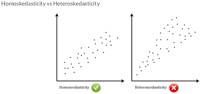
Heteroskedasticity:
- In ancient Greek: "different" (hetero) + "dispersion" (skedasis)
- A time series demonstrates varying volatility systematically over time.
Imports & Settings
import datetime as dt
import sys
import numpy as np
from numpy import cumsum, log, polyfit, sqrt, std, subtract
from numpy.random import randn
import pandas as pd
from pandas_datareader import data as web
import seaborn as sns
from pylab import rcParams
import matplotlib.pyplot as plt
import matplotlib.cm as cm
from arch import arch_model
from numpy.linalg import LinAlgError
from scipy import stats
import statsmodels.api as sm
import statsmodels.tsa.api as tsa
from statsmodels.graphics.tsaplots import plot_acf, plot_pacf
from statsmodels.tsa.stattools import acf, q_stat, adfuller
from sklearn.metrics import mean_squared_error
from scipy.stats import probplot, moment
from arch import arch_model
from arch.univariate import ConstantMean, GARCH, Normal
from sklearn.model_selection import TimeSeriesSplit
import warnings
%matplotlib inline
pd.set_option('display.max_columns', None)
warnings.filterwarnings('ignore')
sns.set(style="darkgrid", color_codes=True)
rcParams['figure.figsize'] = 8,4
Hurst Exponent function
The Hurst Exponent is a statistical measure used to classify time series and infer the level of difficulty in predicting and choosing an appropriate model for the series at hand. The Hurst exponent is used as a measure of long-term memory of time series. It relates to the autocorrelations of the time series, and the rate at which these decrease as the lag between pairs of values increases.
- Value near
0.5indicates a random series. - Value near
0indicates a mean reverting series. - Value near
1indicates a trending series.
def hurst(ts):
    """Returns the Hurst Exponent of the time series vector ts"""
    # Create the range of lag values
    lags = range(2, 100)

    # Calculate the array of the variances of the lagged differences
    tau = [sqrt(std(subtract(ts[lag:], ts[:-lag]))) for lag in lags]

    # Use a linear fit to estimate the Hurst Exponent
    poly = polyfit(log(lags), log(tau), 1)

    # Return the Hurst exponent from the polyfit output
    return poly[0]*2.0
Correlogram Plot
def plot_correlogram(x, lags=None, title=None):
    lags = min(10, int(len(x)/5)) if lags is None else lags
    fig, axes = plt.subplots(nrows=2, ncols=2, figsize=(12, 8))
    x.plot(ax=axes[0][0])
    q_p = np.max(q_stat(acf(x, nlags=lags), len(x))[1])
    stats = f'Q-Stat: {np.max(q_p):>8.2f}\nADF: {adfuller(x)[1]:>11.2f} \nHurst: {round(hurst(x.values),2)}'
    axes[0][0].text(x=.02, y=.85, s=stats, transform=axes[0][0].transAxes)
    probplot(x, plot=axes[0][1])
    mean, var, skew, kurtosis = moment(x, moment=[1, 2, 3, 4])
    s = f'Mean: {mean:>12.2f}\nSD: {np.sqrt(var):>16.2f}\nSkew: {skew:12.2f}\nKurtosis:{kurtosis:9.2f}'
    axes[0][1].text(x=.02, y=.75, s=s, transform=axes[0][1].transAxes)
    plot_acf(x=x, lags=lags, zero=False, ax=axes[1][0])
    plot_pacf(x, lags=lags, zero=False, ax=axes[1][1])
    axes[1][0].set_xlabel('Lag')
    axes[1][1].set_xlabel('Lag')
    fig.suptitle(title, fontsize=20)
    fig.tight_layout()
    fig.subplots_adjust(top=.9)
Download S&P 500 Index Data
We will use daily S&P 500 returns from 2005-2020 to demonstrate the usage of a GARCH model
start = pd.Timestamp('2005-01-01')
end = pd.Timestamp('2020-04-09')

sp_data = web.DataReader('SPY', 'yahoo', start, end)\
      [['High','Low','Open','Close','Volume','Adj Close']]

sp_data.info()
sp_data.head()
Observe volatility clustering
Volatility clustering refers to the observation that "large changes tend to be followed by large changes, of either sign, and small changes tend to be followed by small changes.
- Volatility clustering is frequently observed in financial market data, and it poses a challenge for time series modeling.
with the S&P 500 daily price dataset we calculate daily returns as the percentage price changes, plot the results and observe its behavior over time.
# Calculate daily returns as percentage price changes
sp_data['Return'] = 100 * (sp_data['Close'].pct_change())
sp_data['Log_Return'] = np.log(sp_data['Close']).diff().mul(100) # rescale to faciliate optimization
sp_data = sp_data.dropna()

# Plot ACF, PACF and Q-Q plot and get ADF p-value of series
plot_correlogram(sp_data['Log_Return'], lags=100, title='S&P 500 (Log, Diff)')
plot_correlogram(sp_data['Log_Return'].sub(sp_data['Log_Return'].mean()).pow(2), lags=100, title='S&P 500 Daily Volatility')
Calculate volatility
We compute and convert volatility of price returns in Python.
Firstly, we compute the daily volatility as the standard deviation of price returns. Then convert the daily volatility to monthly and annual volatility.
# Calculate daily std of returns
std_daily = sp_data['Return'].std()
print(f'Daily volatility: {round(std_daily,2)}%')

# Convert daily volatility to monthly volatility
std_monthly = np.sqrt(21) * std_daily
print(f'\nMonthly volatility: {round(std_monthly,2)}%')

# Convert daily volatility to annaul volatility
std_annual = np.sqrt(252) * std_daily
print(f'\nAnnual volatility: {round(std_annual,2)}%')
ARCH and GARCH
First came the ARCH
- Auto Regressive Conditional Heteroskedasticity
- Developed by Robert F. Engle (Nobel prize laureate
2003)
Then came the GARCH
- "Generalized"
ARCH - Developed by Tim Bollerslev (Robert F. Engle's student)
Model notations
Expected return: $$ \mu = Expected|r_t|I(t-1) $$
Expected volatility: $$ \sigma^2 = Expected[(r_t - \mu_t)^2|I(t - 1)] $$
Residual (prediction error): $$ r_t = \mu + \epsilon_t $$
Volatility is related to the residuals: $$ \epsilon_t = \sigma_t * \zeta(WhiteNoise) $$
White noise (z):Uncorrelated random variables with a zero mean and a finite variance
Model intuition
Autoregressive: predict future behavior based on past behavior.- Volatility as a weighted average of past information.
GARCH(1,1) parameter constraints
All parameters are non-negative, so the variance cannot be negative. $$ \omega, \alpha, \beta >= 0 $$
Model estimations are "mean-reverting" to the long-run variance. $$ \alpha + \beta < 1 $$
long-run variance: $$ \omega \: / \: (1 - \alpha - \beta) $$
GARCH(1,1) parameter dynamics
- The larger the
α, the bigger the immediate impact of the shock - The larger the
β, the longer the duration of the impact
Given the GARCH(1,1) model equation as:
Intuitively, GARCH variance forecast can be interpreted as a weighted average of three different variance forecasts.
- One is a constant variance that corresponds to the long run average.
- The second is the new information that was not available when the previous forecast was made.
- The third is the forecast that was made in the previous period.
The weights on these three forecasts determine how fast the variance changes with new information and how fast it reverts to its long run mean.
Simulate ARCH and GARCH series
We will simulate an ARCH(1) and GARCH(1,1) time series respectively using a function simulate_GARCH(n, omega, alpha, beta = 0).
Recall the difference between an ARCH(1) and a GARCH(1,1) model is: besides an autoregressive component of α multiplying lag-1 residual squared, a GARCH model includes a moving average component of β multiplying lag-1 variance.
The function will simulate an ARCH/GARCH series based on n (number of simulations), omega, alpha, and beta (0 by default) you specify. It will return simulated residuals and variances.
def simulate_GARCH(n, omega, alpha, beta = 0):
    np.random.seed(4)
    # Initialize the parameters
    white_noise = np.random.normal(size = n)
    resid = np.zeros_like(white_noise)
    variance = np.zeros_like(white_noise)

    for t in range(1, n):
        # Simulate the variance (sigma squared)
        variance[t] = omega + alpha * resid[t-1]**2 + beta * variance[t-1]
        # Simulate the residuals
        resid[t] = np.sqrt(variance[t]) * white_noise[t]

    return resid, variance
# Simulate a ARCH(1) series
arch_resid, arch_variance = simulate_GARCH(n= 200,
                                           omega = 0.1, alpha = 0.7)
# Simulate a GARCH(1,1) series
garch_resid, garch_variance = simulate_GARCH(n= 200,
                                             omega = 0.1, alpha = 0.7,
                                             beta = 0.1)

# Plot the ARCH variance
plt.figure(figsize=(10,5))
plt.plot(arch_variance, color = 'red', label = 'ARCH Variance')

# Plot the GARCH variance
plt.plot(garch_variance, color = 'orange', label = 'GARCH Variance')
plt.legend()
plt.show()
Observe the impact of model parameters
We will call the function simulate_GARCH() again, and study the impact of GARCH model parameters on simulated results.
Specifically, we will simulate two GARCH(1,1) time series, they have the same omega and alpha, but different beta as input.
Recall in GARCH(1,1), since β is the coefficient of lag-1 variance, if the α is fixed, the larger the β, the longer the duration of the impact. In other words, high or low volatility periods tend to persist. Pay attention to the plotted results and see whether we can verify the β impact.
# First simulated GARCH
plt.figure(figsize=(10,3))
sim_resid, sim_variance = simulate_GARCH(n = 200,  omega = 0.1, alpha = 0.3, beta = 0.2)
plt.plot(sim_variance, color = 'orange', label = 'Variance')
plt.plot(sim_resid, color = 'green', label = 'Residuals')
plt.title('First simulated GARCH, Beta = 0.2')
plt.legend(loc='best')
plt.show()

# Second simulated GARCH
plt.figure(figsize=(10,3))
sim_resid, sim_variance = simulate_GARCH(n = 200,  omega = 0.1, alpha = 0.3, beta = 0.6)
plt.plot(sim_variance, color = 'red', label = 'Variance')
plt.plot(sim_resid, color = 'deepskyblue', label = 'Residuals')
plt.title('Second simulated GARCH, Beta = 0.6')
plt.legend(loc='best')
plt.show()
Implement a basic GARCH model
We will get familiar with the Python arch package, and use its functions such as arch_model() to implement a GARCH(1,1) model.
First define a basic GARCH(1,1) model, then fit the model, review the model fitting summary, and plot the results.
# Specify GARCH model assumptions
basic_gm = arch_model(sp_data['Return'], p = 1, q = 1,
                      mean = 'constant', vol = 'GARCH', dist = 'normal')
# Fit the model
gm_result = basic_gm.fit(update_freq = 4)
# Display model fitting summary
print(gm_result.summary())
# Plot fitted results
gm_result.plot()
plt.show()
Make forecast with GARCH models
We will practice making a basic volatility forecast.
We will call .forecast() to make a prediction. By default it produces a 1-step ahead estimate. You can use horizon = n to specify longer forward periods.
# Make 5-period ahead forecast
gm_forecast = gm_result.forecast(horizon = 5)

# Print the forecast variance
print(gm_forecast.variance[-1:])
h.1 in row "2020-04-09": is a 1-step ahead forecast made using data up to and including that date
Distribution assumptions
Why make assumptions?
- Volatility is not directly observable
- GARCH model use residuals as volatility shocks $$ r_t = \mu + t + \epsilon_t $$
- Volatility is related to the residuals: $$ \epsilon_t = \sigma_t * \zeta(WhiteNoise) $$
Standardized residuals
- Residual = predicted return - mean return $$ residuals = \epsilon_t = r_t - \mu_t $$
- Standardized residual = residual / return volatility $$ std Resid = \frac{\epsilon_t}{\sigma_t} $$
GARCH models make distribution assumptions about the residuals and the mean return. Financial time series data often does not follow a normal distribution. In financial time series it is much more likely to observe extreme positive and negative values that are far away from the mean. to improve a GARCH models distribution assumptions to be more representative of real financial data we can specify the models distribution assumption to be a Student's t-distribution. A Student's t-distribution is symmetric and bell shaped similar to a normal distribution but has fatter tails making it more prone to producing values that fall far away from its mean. The nu $(\nu)$ parameter indicates its shape the larger the $\nu$ the more peaked the curve becomes.
GARCH models enable one to specify the distribution assumptions of the standardized residuals. By default, a normal distribution is assumed, which has a symmetric, bell-shaped probability density curve. Other options include Student's t-distribution and skewed Student's t-distribution.
Plot distribution of standardized residuals
We will practice computing the standardized residuals from a fitted GARCH model, and then plot its histogram together with a normal fit distribution normal_resid.
# Obtain model estimated residuals and volatility
gm_resid = gm_result.resid
gm_std = gm_result.conditional_volatility

# Calculate the standardized residuals
gm_std_resid = gm_resid /gm_std

# Plot the histogram of the standardized residuals
plt.figure(figsize=(7,4))
sns.distplot(gm_std_resid, norm_hist=True, fit=stats.norm, bins=50, color='r')
plt.legend(('normal', 'standardized residuals'))
plt.show()
Fit a GARCH with skewed t-distribution
We will improve the GARCH model by using a skewed Student's t-distribution assumption. In addition.
# Specify GARCH model assumptions
skewt_gm = arch_model(sp_data['Return'], p = 1, q = 1, mean = 'constant', vol = 'GARCH', dist = 'skewt')

# Fit the model
skewt_result = skewt_gm.fit(disp = 'off')

# Get model estimated volatility
skewt_vol = skewt_result.conditional_volatility
# Plot model fitting results
plt.plot(skewt_vol, color = 'red', label = 'Skewed-t Volatility')
plt.plot(sp_data['Return'], color = 'grey',
         label = 'Daily Returns', alpha = 0.4)
plt.legend(loc = 'upper right')
plt.show()
Mean model specifications
Constant mean: generally works well with most financial return data.
Autoregressive mean: model the mean as an autoregressive (AR) process.
Zero mean: Use when the mean has been modeled separately to fit the residuals of the separate model to estimate volatility (preferred method).
Here we model the log-returns of the S&P 500 data with an ARMA model and then fit the models residuals to estimate the volatility of the returns series with a GARCHmodel.
Searching over model orders to find the optimal number of lags
import pmdarima as pm

model = pm.auto_arima(sp_data['Log_Return'],

d=0, # non-seasonal difference order
start_p=1, # initial guess for p
start_q=1, # initial guess for q
max_p=4, # max value of p to test
max_q=4, # max value of q to test

seasonal=False, # is the time series seasonal

information_criterion='bic', # used to select best model
trace=True, # print results whilst training
error_action='ignore', # ignore orders that don't work
stepwise=True, # apply intelligent order search

)
print(model.summary())
# Fit best model
_arma_model = sm.tsa.SARIMAX(endog=sp_data['Log_Return'],order=(0, 0, 1))
_model_result = _arma_model.fit()
# Plot model residuals
_model_result.plot_diagnostics(figsize=(10, 5))
plt.show()
# Fit GARCH model with ARMA model residuals
_garch_model = arch_model(_model_result.resid, mean='Zero', p=1, q=1)
_garch_result = _garch_model.fit(disp = 'off')
print(_garch_result.summary())
# Plot GARCH model fitted results
_garch_result.plot()
plt.show()
plot_correlogram(_garch_result.resid.dropna(), lags=100, title='GARCH Residuals')
Modeling of asymmetric responses of volatility
Leverage effect
- Debt-equity Ratio = Debt / Equity
- Stock price goes down, debt-equity ratio goes up
- Riskier!
GARCH models assume positive and negative news has a symmetric impact on volatility. However, in reality the market tends to take the stairs up and the elevator down. In other words, the impact is usually asymmetric, and negative news tends to affect the volatility more than positive news.
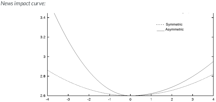
GARCH models that account for asymmetric shocks:
GJR-GARCH- A popular option to model asymmetric shocks
- GJR-GARCH in Python:
arch_model(my_data, p = 1, q = 1, o = 1, mean = 'constant', vol = 'GARCH')
$$ \sigma_t^2 = \omega + (\alpha + \gamma I_{t-1} + \beta \sigma_{t-1}^2 $$ $$ I_{t-1} := \begin{cases} 0 \text{ if } r_{t-1} \geq \mu \\ 1 \text{ if } r_{t-1} < \mu \end{cases}$$
EGARCH- Exponential GARCH
- Add a conditional component to model the asymmetry in shocks similar to the GJR-GARCH
- No non-negative constraints on alpha, beta so it runs faster
- GJR-GARCH in Python:
arch_model(my_data, p = 1, q = 1, o = 1, mean = 'constant', vol = EGARCH)
$$ log \: \sigma_t^2 = \omega + \sum_{k=1}^q \beta_k g (Z_t - k) + \sum_{k=1}^p \alpha_k \: log \: \sigma_{t-k}^2 $$
where $ g(Z_t) = \theta Z_t + \lambda(|Z_t| - E(|Z_t|)), \sigma_t^2 $ is the conditional variance, $\omega,\beta, \alpha, \theta \text{ and } \lambda$ are coefficients.
Fit GARCH models to cryptocurrency
Financial markets tend to react to positive and negative news shocks very differently, and one example is the dramatic swings observed in the cryptocurrency market in recent years.
We will implement a GJR-GARCH and an EGARCH model respectively in Python, which are popular choices to model the asymmetric responses of volatility.
Load the daily Bitcoin price from the Blockchain.com API:
bitcoin_data = pd.read_csv('https://api.blockchain.info/charts/market-price?start=2010-10-09×pan=12years&format=csv',
names=['Timestamp','Close'], index_col='Timestamp')
bitcoin_data.index = pd.to_datetime(bitcoin_data.index, format='%Y-%m-%d')
bitcoin_data = bitcoin_data.loc[(bitcoin_data != 0.0).any(axis=1)]
bitcoin_data['Return'] = np.log(bitcoin_data['Close']).diff().mul(100) # rescale to faciliate optimization
bitcoin_data = bitcoin_data.dropna()
bitcoin_data.info()
# Plot bitcoin price data
fig, ax1 = plt.subplots(figsize=(13, 5))
ax1.set_yscale('log')
ax1.plot(bitcoin_data.index, bitcoin_data.Close, color='b', label='BTCUSD')
ax1.set_xlabel('Date')
ax1.set_ylabel('BTCUSD Close')
ax1.legend()
plt.show()
plot_correlogram(bitcoin_data['Return'], lags=100, title='BTCUSD (Log, Diff)')
plot_correlogram(bitcoin_data['Return'].sub(bitcoin_data['Return'].mean()).pow(2), lags=100, title='BTCUSD Daily Volatility')
# Specify GJR-GARCH model assumptions
gjr_gm = arch_model(bitcoin_data['Return'], p = 1, q = 1, o = 1, vol = 'GARCH', dist = 't')

# Fit the model
gjrgm_result = gjr_gm.fit(disp = 'off')

# Print model fitting summary
print(gjrgm_result.summary())
# Specify EGARCH model assumptions
egarch_gm = arch_model(bitcoin_data['Return'], p = 1, q = 1, o = 1, vol = 'EGARCH', dist = 't')

# Fit the model
egarch_result = egarch_gm.fit(disp = 'off')

# Print model fitting summary
print(egarch_result.summary())
Compare GJR-GARCH with EGARCH
Previously we fitted a GJR-GARCH and EGARCH model with Bitcoin return time series. Now we will compare the estimated conditional volatility from the two models by plotting their results.
gjrgm_vol = gjrgm_result.conditional_volatility
egarch_vol = egarch_result.conditional_volatility

# Plot the actual Bitcoin returns
plt.plot(bitcoin_data['Return'], color = 'grey', alpha = 0.4, label = 'Price Returns')

# Plot GJR-GARCH estimated volatility
plt.plot(gjrgm_vol, color = 'blue', label = 'GJR-GARCH Volatility')

# Plot EGARCH  estimated volatility
plt.plot(egarch_vol, color = 'red', label = 'EGARCH Volatility')

plt.legend(loc = 'upper right')
plt.show()
# Print each models BIC
print(f'GJR-GARCH BIC: {gjrgm_result.bic}')
print(f'\nEGARCH BIC: {egarch_result.bic}')
Overall both GJR-GARCH and EGARCH models did a good job of fitting the actual data. Comparatively, GJR-GARCH is more conservative in volatility estimation when applying it to the Bitcoin dataset, but EGARCH yields the better model.
GARCH rolling window forecast
- Expanding window forecast: Continuously add new data points to the sample.
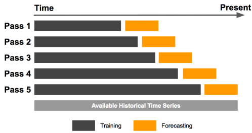
- Fixed rolling window forecast: New data points are added while old ones are dropped from the sample.
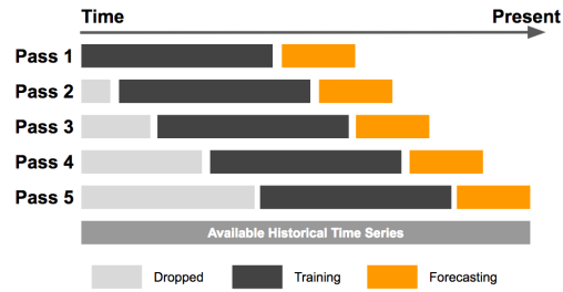
- Rolling window forecast
- Avoids lookback bias
- Less subject to overfitting
- Adapt forecast to new observations
How to determine window size ?
- Usually determined on a case-by-case basis.
- Too wide window size: include obsolete data that may lead to high bias.
- Too narrow window size: exclude relevant data that may lead to higher variance.
- The optimal window size: trade-off to balance bias and variance.
Fixed rolling window forecast
Rolling-window forecasts are very popular for financial time series modeling. We will practice how to implement GARCH model forecasts with a fixed rolling window.
First define the window size inside .fit(), and perform the forecast with a for-loop. Note since the window size remains fixed, both the start and end points increment after each iteration.
index = sp_data.index
start_loc = 0
end_loc = np.where(index >= '2020-1-1')[0].min()
forecasts = {}
for i in range(70):
    sys.stdout.write('-')
    sys.stdout.flush()
    res = _garch_model.fit(first_obs=start_loc + i, last_obs=i + end_loc, disp='off')
    temp = res.forecast(horizon=1).variance
    fcast = temp.iloc[i + end_loc - 1]
    forecasts[fcast.name] = fcast
print(' Done!')
variance_fixedwin = pd.DataFrame(forecasts).T
Implement expanding window forecast
index = sp_data.index
start_loc = 0
end_loc = np.where(index >= '2020-1-1')[0].min()
forecasts = {}
for i in range(70):
    sys.stdout.write('-')
    sys.stdout.flush()
    res = _garch_model.fit(first_obs = start_loc, last_obs = i + end_loc, disp = 'off')
    temp = res.forecast(horizon=1).variance
    fcast = temp.iloc[i + end_loc - 1]
    forecasts[fcast.name] = fcast
print(' Done!')
variance_expandwin = pd.DataFrame(forecasts).T
Compare forecast results
Different rolling window approaches can generate different forecast results. Here we will take a closer look by comparing these forecast results.
# Calculate volatility from variance forecast with an expanding window
vol_expandwin = np.sqrt(variance_expandwin)

# Calculate volatility from variance forecast with a fixed rolling window
vol_fixedwin = np.sqrt(variance_fixedwin)

# Plot results
plt.figure(figsize=(10,5))

# Plot volatility forecast with an expanding window
plt.plot(vol_expandwin, color = 'blue', label='Expanding Window')

# Plot volatility forecast with a fixed rolling window
plt.plot(vol_fixedwin, color = 'red', label='Rolling Window')

plt.plot(sp_data.Return.loc[variance_expandwin.index], color = 'grey', label='Daily Return')

plt.legend()
plt.show()
Simplify the model with p-values
Leonardo da Vinci once said: "Simplicity is the ultimate sophistication." It also applies to data science modeling. We will practice using the p-values to decide the necessity of model parameters, and define a parsimonious model without insignificant parameters.
The null hypothesis is the parameter value is zero. If the p-value is larger than a given confidence level, the null hypothesis cannot be rejected, meaning the parameter is not statistically significant, hence not necessary.
# Get parameter stats from model summary
para_summary = pd.DataFrame({'parameter':gm_result.params,
                             'p-value': gm_result.pvalues})

# Print out parameter stats
print(para_summary)
Simplify the model with t-statistics
Besides p-values, t-statistics can also help decide the necessity of model parameters. We will practice using t-statistics to assess the significance of model parameters.
Whats a T-statistic?
The t-statistic is computed as the estimated parameter value subtracted by its expected mean (zero in this case), and divided by its standard error. The absolute value of the t-statistic is a distance measure, that tells you how many standard errors the estimated parameter is away from 0. As a rule of thumb, if the t-statistic is larger than 2, you can reject the null hypothesis.
# Get parameter stats from model summary
para_summary = pd.DataFrame({'parameter':gm_result.params,
                             'std-err': gm_result.std_err,
                             't-value': gm_result.tvalues})

# Verify t-statistic by manual calculation
calculated_t = para_summary['parameter']/para_summary['std-err']

# Print parameter stats
print(para_summary)
Ljung-Box test
The Ljung-Box tests whether any of a group of autocorrelations of a time series are different from zero.
- H0: the data is independently distributed
- P-value <
5%: the model is not sound
We will practice detecting autocorrelation in the standardized residuals by performing a Ljung-Box test.
The null hypothesis of Ljung-Box test is: the data is independently distributed. If the p-value is larger than the specified significance level, the null hypothesis cannot be rejected. In other words, there is no clear sign of autocorrelations and the model is valid.
# Import the Python module
from statsmodels.stats.diagnostic import acorr_ljungbox

# Perform the Ljung-Box test
lb_test = acorr_ljungbox(gm_std_resid , lags = 10)

# Store p-values in DataFrame
df = pd.DataFrame({'P-values': lb_test[1]}).T

# Create column names for each lag
col_num = df.shape[1]
col_names = ['lag_'+str(num) for num in list(range(1,col_num+1,1))]

# Display the p-values
df.columns = col_names
df
# Display the significant lags
mask = df < 0.05
df[mask].dropna(axis=1)
Goodness of fit
Can model do a good job explaining the data?
Maximum likelihoodInformation criteria (AIC, BIC)
Maximum likelihood: Maximize the probability of getting the data observed under the assumed model. Preferred models have larger likelihood values.
Maximum likelihood estimation:
In statistics, maximum likelihood estimation (MLE) is a method of estimating the parameters of a probability distribution by maximizing a likelihood function, so that under the assumed statistical model the observed data is most probable. The point in the parameter space that maximizes the likelihood function is called the maximum likelihood estimate.
Likelihood function:
In statistics, the likelihood function (often simply called the likelihood) measures the goodness of fit of a statistical model to a sample of data for given values of the unknown parameters. It is formed from the joint probability distribution of the sample, but viewed and used as a function of the parameters only, thus treating the random variables as fixed at the observed values. The likelihood function describes a hypersurface whose peak, if it exists, represents the combination of model parameter values that maximize the probability of drawing the sample obtained.
Pick a winner based on log-likelihood
We will practice using log-likelihood to choose a model with the best fit.
# Print the log-likelihodd of normal GARCH
print('Log-likelihood of normal GARCH :', gm_result.loglikelihood)
# Print the log-likelihodd of skewt GARCH
print('Log-likelihood of skewt GARCH :', skewt_result.loglikelihood)
Backtesting with MAE, MSE
We will practice how to evaluate model performance by conducting backtesting. The out-of-sample forecast accuracy is assessed by calculating MSE and MAE.
from sklearn.metrics import mean_absolute_error, mean_squared_error
def evaluate(observation, forecast):
    # Call sklearn function to calculate MAE
    mae = mean_absolute_error(observation, forecast)
    print(f'Mean Absolute Error (MAE): {round(mae,3)}')
    # Call sklearn function to calculate MSE
    mse = mean_squared_error(observation, forecast)
    print(f'Mean Squared Error (MSE): {round(mse,3)}')
    return mae, mse

# Backtest model with MAE, MSE
evaluate(bitcoin_data['Return'].sub(bitcoin_data['Return'].mean()).pow(2), egarch_vol**2)
# Plot the actual Bitcoin volatility
plt.plot(bitcoin_data['Return'].sub(bitcoin_data['Return'].mean()).pow(2),
         color = 'grey', alpha = 0.4, label = 'Daily Volatility')

# Plot EGARCH  estimated volatility
plt.plot(egarch_vol**2, color = 'red', label = 'EGARCH Volatility')

plt.legend(loc = 'upper right')
plt.show()
Simulating Forecasts
When using simulation- or bootstrap-based forecasts, an additional attribute of an ARCHModelForecast object is meaningful – simulation.
Bootstrap Forecasts
Bootstrap-based forecasts are nearly identical to simulation-based forecasts except that the values used to simulate the process are computed from historical data rather than using the assumed distribution of the residuals. Forecasts produced using this method also return an ARCHModelForecastSimulation containing information about the simulated paths.
# The paths for the final observation
sim_forecasts = egarch_result.forecast(horizon=5, method='simulation')
sim_paths = sim_forecasts.simulations.residual_variances[-1].T
sim = sim_forecasts.simulations

bs_forecasts = egarch_result.forecast(horizon=5, method='bootstrap')
bs_paths = bs_forecasts.simulations.residual_variances[-1].T
bs = bs_forecasts.simulations
Comparing the paths
The paths are available on the attribute simulations. Plotting the paths shows important differences between the two scenarios beyond the average differences. Both start at the same point.
fig, axes = plt.subplots(1, 2, figsize=(13,5))

x = np.arange(1, 6)

# Plot the paths and the mean, set the axis to have the same limit
axes[0].plot(x, np.sqrt(252 * sim_paths), color='tomato', alpha=0.2)
axes[0].plot(x, np.sqrt(252 * sim_forecasts.residual_variance.iloc[-1]),
    color='k', alpha=1)

axes[0].set_title('Model-based Simulation')
axes[0].set_xticks(np.arange(1, 6))
axes[0].set_xlim(1, 5)

axes[1].plot(x, np.sqrt(252 * bs_paths), color='deepskyblue', alpha=0.2)
axes[1].plot(x,np.sqrt(252 * bs_forecasts.residual_variance.iloc[-1]),
    color='k', alpha=1)

axes[1].set_xticks(np.arange(1, 6))
axes[1].set_xlim(1, 5)

axes[1].set_title('Bootstrap Scenario')
plt.show()
# Plot Simulation Variances
fig, axes = plt.subplots(1, 2, figsize=(13,5))

sns.boxplot(data=sim.variances[-1], ax=axes[0])
sns.boxplot(data=bs.variances[-1], ax=axes[1])

axes[0].set_title('Model-based Simulation Variances')
axes[1].set_title('Bootstrap Simulation Variances')

plt.show()
VaR in financial risk management
What is VaR? VaR stands for Value at Risk
Three ingredients:
- portfolio
- time horizon
- probability
VaR examples
1-day 5% VaR of $1 million
- 5% probability the portfolio will fall in value by 1 million dollars or more over a 1-day period
10-day 1% VaR of $9 million
- 1% probability the portfolio will fall in value by 9 million dollars or more over a 10-day period
VaR in risk management
- Set risk limits
- VaR exceedance: portfolio loss exceeds the VaR
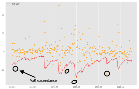
Suppose a 5% daily VaR and 252 trading days in a year. A valued VaR model should have less than 13 VaR exceedance in a year, that is 5% * 252 if there are more exceedances the model is under estimating the risk.
Dynamic VaR with GARCH
- More realistic VaR estimation with GARCH
- VaR =
mean + (GARCH vol) * quantile
Parametric VaR
- Estimate quantiles based on GARCH assumed distribution of the standardized residuals.
Empirical VaR
- Estimate quantiles based on the observed distribution of the GARCH standardized residuals.
Compute parametric VaR
We will practice estimating dynamic 5% and 1% daily VaRs with a parametric approach.
Recall there are three steps to perform a forward VaR estimation. Step 1 is to use a GARCH model to make variance forecasts. Step 2 is to obtain the GARCH forward-looking mean and volatility. And Step 3 is to compute the quantile according to a given confidence level. The parametric approach estimates quantiles from an assumed distribution assumption.
am = arch_model(bitcoin_data['Return'], p = 1, q = 1, o = 1, vol = 'EGARCH', dist = 't')
res = am.fit(disp='off', last_obs='2018-01-01')
forecasts = res.forecast(start='2019-01-01')
cond_mean = forecasts.mean['2019':]
cond_var = forecasts.variance['2019':]
q = am.distribution.ppf([0.01, 0.05], res.params[5])
print(q)
value_at_risk = -cond_mean.values - np.sqrt(cond_var).values * q[None, :]
value_at_risk = pd.DataFrame(value_at_risk, columns=['1%', '5%'], index=cond_var.index)
value_at_risk.describe()
ax = value_at_risk.plot(legend=False, figsize=(12,6))
xl = ax.set_xlim(value_at_risk.index[0], value_at_risk.index[-1])

rets_2019 = bitcoin_data.Return['2019':]
rets_2019.name = 'BTCUSD Return'

c = []
for idx in value_at_risk.index:
    if rets_2019[idx] > -value_at_risk.loc[idx, '5%']:
        c.append('#000000')
    elif rets_2019[idx] < -value_at_risk.loc[idx, '1%']:
        c.append('#BB0000')
    else:
        c.append('#BB00BB')

c = np.array(c, dtype='object')

labels = {

    '#BB0000': '1% Exceedence',
    '#BB00BB': '5% Exceedence',
    '#000000': 'No Exceedence'
}

markers = {'#BB0000': 'x', '#BB00BB': 's', '#000000': 'o'}

for color in np.unique(c):
    sel = c == color
    ax.scatter(
        rets_2019.index[sel],
        -rets_2019.loc[sel],
        marker=markers[color],
        c=c[sel],
        label=labels[color])

ax.set_title('Parametric VaR')
ax.legend(frameon=False, ncol=3)

plt.show()
Compute empirical VaR
We will practice estimating dynamic 5% and 1% daily VaRs with an empirical approach.
The difference between parametric VaR and empirical VaR is how the quantiles are estimated. The parametric approach estimates quantiles from an assumed distribution assumption, while the empirical approach estimates quantiles from an observed distribution of the standardized residuals.
# Obtain model estimated residuals and volatility
gm_resid = res.resid
gm_std = res.conditional_volatility

# Calculate the standardized residuals
gm_std_resid = gm_resid /gm_std

# Obtain the empirical quantiles
q = gm_std_resid.quantile([.01, .05])
print(q)
value_at_risk = -cond_mean.values - np.sqrt(cond_var).values * q.values[None, :]
value_at_risk = pd.DataFrame(value_at_risk, columns=['1%', '5%'], index=cond_var.index)
value_at_risk.describe()
ax = value_at_risk.plot(legend=False, figsize=(12,6))
xl = ax.set_xlim(value_at_risk.index[0], value_at_risk.index[-1])

rets_2019 = bitcoin_data.Return['2019':]
rets_2019.name = 'BTCUSD Return'

c = []
for idx in value_at_risk.index:
    if rets_2019[idx] > -value_at_risk.loc[idx, '5%']:
        c.append('#000000')
    elif rets_2019[idx] < -value_at_risk.loc[idx, '1%']:
        c.append('#BB0000')
    else:
        c.append('#BB00BB')

c = np.array(c, dtype='object')
for color in np.unique(c):
    sel = c == color
    ax.scatter(
        rets_2019.index[sel],
        -rets_2019.loc[sel],
        marker=markers[color],
        c=c[sel],
        label=labels[color])

ax.set_title('Filtered Historical Simulation VaR')
ax.legend(frameon=False, ncol=3)

plt.show()
Plot the 5% daily VaR with the price
fig, ax1 = plt.subplots(figsize=(13, 5))
ax2 = ax1.twinx()

ax1.grid(False)
ax2.grid(False)

ax1.plot(bitcoin_data.loc[value_at_risk.index[0]:].index, bitcoin_data.loc[value_at_risk.index[0]:].Close,
         color='red', label='BTCUSD')
ax2.plot(value_at_risk['5%'].index, value_at_risk['5%'], color='grey', label='VaR', alpha=0.5)

ax1.set_xlabel('Date')
ax1.set_ylabel('BTCUSD Close')
ax2.set_ylabel('VaR')

ax1.legend(loc='upper left')
ax2.legend()

plt.show()
What is covariance?
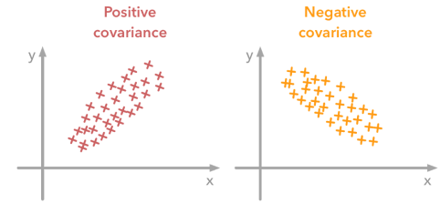
- Describe the relationship between movement of two variables.
- Positive covariance: move together.
- Negative covariance; move in the opposite directions.
Dynamic covariance with GARCH
If two asset returns have correlation ρ and time-varying volatility of σ 1 and σ 2 : $ Covariance = p * \sigma_1 * \sigma_2 $
Compute GARCH covariance
We will practice computing dynamic covariance with GARCH models.
Download Price Data
start = pd.Timestamp('2012-01-01')
end = pd.Timestamp('2020-01-06')

sp_data = web.DataReader('SPY', 'yahoo', start, end)\
      [['High','Low','Open','Close','Volume','Adj Close']]

sp_data.info()
tmf_data = web.DataReader('TMF', 'yahoo', start, end)\
      [['High','Low','Open','Close','Volume','Adj Close']]

tmf_data.info()
upro_data = web.DataReader('UPRO', 'yahoo', start, end)\
      [['High','Low','Open','Close','Volume','Adj Close']]

upro_data.info()
Plot Price Data
prices = pd.DataFrame({'UPRO': upro_data['Close'],
                       'SPY': sp_data['Close'],
                       'TMF': tmf_data['Close']})

prices.div(prices.iloc[0,:]).plot(figsize=(12, 6))# Normalize Prices
Calculate Returns
tmf_data['Return'] = np.log(tmf_data['Close']).diff().mul(100) # rescale to faciliate optimization
tmf_data = tmf_data.dropna()

upro_data['Return'] = np.log(upro_data['Close']).diff().mul(100) # rescale to faciliate optimization
upro_data = upro_data.dropna()

sp_data['Return'] = np.log(sp_data['Close']).diff().mul(100) # rescale to faciliate optimization
sp_data = sp_data.dropna()
Find best Model
sp_model = pm.auto_arima(sp_data['Return'],

d=0, # non-seasonal difference order
start_p=1, # initial guess for p
start_q=1, # initial guess for q
max_p=4, # max value of p to test
max_q=4, # max value of q to test

seasonal=False, # is the time series seasonal

information_criterion='bic', # used to select best model
trace=True, # print results whilst training
error_action='ignore', # ignore orders that don't work
stepwise=True, # apply intelligent order search

)
print(sp_model.summary())
tmf_model = pm.auto_arima(tmf_data['Return'],

d=0, # non-seasonal difference order
start_p=1, # initial guess for p
start_q=1, # initial guess for q
max_p=4, # max value of p to test
max_q=4, # max value of q to test

seasonal=False, # is the time series seasonal

information_criterion='bic', # used to select best model
trace=True, # print results whilst training
error_action='ignore', # ignore orders that don't work
stepwise=True, # apply intelligent order search

)
print(tmf_model.summary())
upro_model = pm.auto_arima(upro_data['Return'],

d=0, # non-seasonal difference order
start_p=1, # initial guess for p
start_q=1, # initial guess for q
max_p=4, # max value of p to test
max_q=4, # max value of q to test

seasonal=False, # is the time series seasonal

information_criterion='bic', # used to select best model
trace=True, # print results whilst training
error_action='ignore', # ignore orders that don't work
stepwise=True, # apply intelligent order search

)
print(upro_model.summary())
Fit best Model
_arma_sp = sm.tsa.SARIMAX(endog=sp_data['Return'],order=(0, 0, 0))
_sp_model_result = _arma_sp.fit()

egarch_sp = arch_model(_sp_model_result.resid, p = 1, q = 1, o = 1, vol = 'EGARCH', dist = 't', mean = 'zero')
sp_gm_result = egarch_sp.fit(disp = 'off')
print(sp_gm_result.summary())
_arma_tmf = sm.tsa.SARIMAX(endog=tmf_data['Return'],order=(0, 0, 0))
_tmf_model_result = _arma_tmf.fit()

egarch_tmf = arch_model(_tmf_model_result.resid, p = 1, q = 1, o = 1, vol = 'EGARCH', dist = 't', mean = 'zero')
tmf_gm_result = egarch_tmf.fit(disp = 'off')
print(tmf_gm_result.summary())
_arma_upro = sm.tsa.SARIMAX(endog=upro_data['Return'],order=(0, 0, 0))
_upro_model_result = _arma_upro.fit()

egarch_upro = arch_model(_upro_model_result.resid, p = 1, q = 1, o = 1, vol = 'EGARCH', dist = 't', mean = 'zero')
upro_gm_result = egarch_upro.fit(disp = 'off')
print(upro_gm_result.summary())
# Step 1: Fit GARCH models and obtain volatility for each return series
vol_tmf = tmf_gm_result.conditional_volatility
vol_upro = upro_gm_result.conditional_volatility
# Step 2: Compute standardized residuals from the tted GARCH models
resid_tmf = tmf_gm_result.resid/vol_tmf
resid_upro = upro_gm_result.resid/vol_upro
# Step 3: Compute ρ as simple correlation of standardized residuals
corr = np.corrcoef(resid_tmf, resid_upro)[0,1]
# Step 4: Compute GARCH covariance by multiplying the correlation and volatility.
covariance = corr * vol_tmf * vol_upro
# Plot the data
plt.plot(covariance, color = 'red')
plt.title('GARCH Covariance')
plt.show()
Compute dynamic portfolio variance
We will practice computing the variance of a simple two-asset portfolio with GARCH dynamic covariance.
The Modern Portfolio Theory states that there is an optimal way to construct a portfolio to take advantage of the diversification effect, so one can obtain a desired level of expected return with the minimum risk. This effect is especially evident when the covariance between asset returns is negative.
Find best max sharpe ratio weights
data = {}
for perc in range(100):
    daily = (1 - perc / 100) * tmf_data["Return"] + (perc / 100) * upro_data["Return"]
    data[perc] = daily.mean() / daily.std() * (252 ** 0.5)

sx = pd.Series(data)
s = pd.DataFrame(sx, index=sx.index)
ax = s.plot(title="UPRO/TMF allocation vs Sharpe")
ax.set_ylabel("Sharpe Ratio")
ax.set_xlabel("Percent Portfolio UPRO")
plt.show()

tmf_w = 100 - s.idxmax()[0]
print('Optimal UPRO Weight =', s.idxmax()[0])
print('Optimal TNF Weight =', tmf_w)
print('Optimal Sharpe Ratio =', s.max()[0])
# Define weights
Wa1 = 0.64
Wa2 = 0.36

Wb1 = 0.49
Wb2 = 1 - Wb1

# Calculate individual returns variance
variance_upro = np.var(upro_data['Return'])
variance_tmf = np.var(tmf_data['Return'])

# Calculate portfolio variance
portvar_a = Wa1**2 * variance_tmf + Wa2**2 * variance_upro + 2*Wa1*Wa2*covariance
portvar_b = Wb1**2 * variance_tmf + Wb2**2 * variance_upro + 2*Wb1*Wb2*covariance

# Plot the data
plt.plot(portvar_a, color = 'red', label = 'Portfolio a')
plt.plot(portvar_b, color = 'deepskyblue', label = 'Portfolio b')
plt.title('Covariance')
plt.legend(loc = 'best')
plt.show()
What is Beta?
Stock Beta: A measure of stock volatility in relation to the general market.
Systematic risk: The portion of the risk that cannot be diversified away.
Beta in portfolio management
- Gauge investment risk
Market Beta = 1:used as benchmarkBeta > 1:the stock bears more risks than the general marketBeta < 1:the stock bears less risks than the general market
Dynamic Beta with GARCH $$ Beta = p * \frac{\sigma_{stock}}{\sigma_{market}} $$
# 1). Compute correlation between S&P500 and stock
resid_stock = tmf_gm_result.resid / tmf_gm_result.conditional_volatility
resid_sp500 = sp_gm_result.resid / sp_gm_result.conditional_volatility

correlation = np.corrcoef(resid_stock, resid_sp500)[0, 1]

# 2). Compute dynamic Beta for the stock
stock_beta = correlation * (tmf_gm_result.conditional_volatility / sp_gm_result.conditional_volatility)
# Plot the Beta
plt.title('TMF Stock Beta')
plt.plot(stock_beta)
plt.show()